2 Welcome to R
Toronto, Ontario has an open data portal. As with such portals in many other cities, the goal was to put the data in the hands of people who might do something with them. The data available there are quite diverse in their content, enabling analyses on all nature of question. For those interested in homelessness, there are daily occupancy numbers for shelters; for those interested in housing, Airbnb rental registrations; for those interested in climate change, a survey on Torontonians’ climate perceptions; for transportation enthusiasts, the locations of bus stops, train stops, and the sidewalk network; for political watchers, election results by ward; for those interested in local economics, all licenses for businesses operating in the city. And, of course, 311 requests are available for download, documenting where and when Torontonians have identified graffiti, potholes, street light outages, and other local needs.
While the breadth and organization of the data on Toronto’s open data portal are noteworthy, what really sets it apart is something additional the City did to facilitate use of the data. They worked with Sharla Gelfand, a local developer, to build a custom package for R statistical software—or ‘R,’ for short—that facilitates browsing and downloading the data, called opendatatoronto (Gelfand 2020) (also see Figure 2.1) . The practical upshot is that statisticians, analysts, visualizers, hackers, and researchers who use R—which is one of the most popular softwares for accessing, managing, and analyzing data—can access data from Toronto’s Open Data Portal from within the program, without having to go through the tedious process of manually visiting the web site, browsing data sets, downloading data, and then loading them into R. How convenient! So much so that Toronto has not been alone in this idea. Numerous metro transit systems, including Washington, D.C., have done the same for their data. A developer in Vancouver, British Columbia, built one called, fittingly, VancouvR (von Bergmann 2021) . And Socrata , the biggest vendor of municipal open data portals has one called RSocrata (Devlin et al. 2021) that generalizes to all data portals they have built.
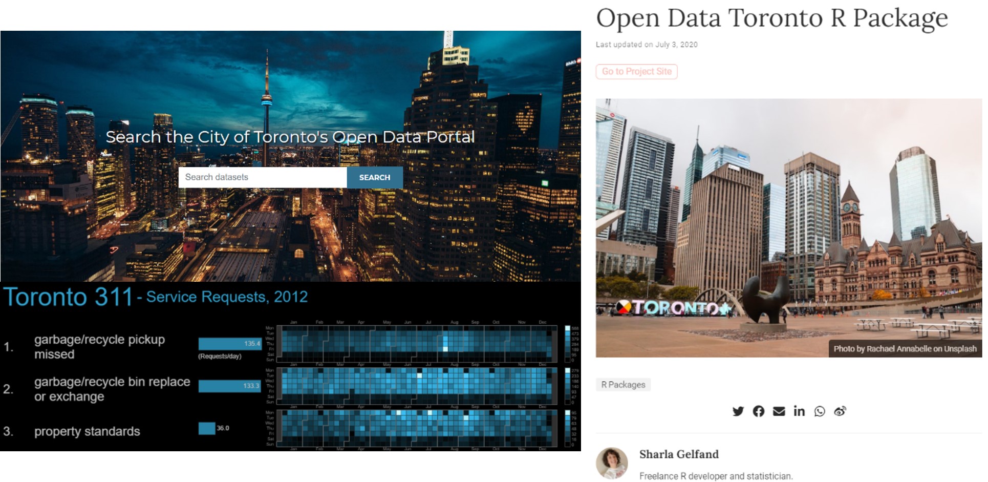
Figure 2.1: The City of Toronto’s Open Data Portal (top left) is accompanied by an R package designed to directly access its contents, opendatatoronto (right), and also has a gallery featuring ways in which people have used the data, including this visualization of the most common 311 reports by day across the year. (Credit: https://open.toronto.ca/, https://www.sharlagelfand.com/project/opendatatoronto/, http://neoformix.com/Projects/Toronto311/)
This anecdote illustrates just how central R has become to urban informatics and data science in general, which is owed to a few distinctive characteristics. R is free to download and install. It has a very approachable and flexible programming language. Further, developers can use that language to build new “packages”—what you might think of as “add-ons” or “plug-ins”—that offer new capabilities not available in the original software, which is exactly what the City of Toronto and Sharla Gelfand did.
2.1 Worked Example and Learning Objectives
Just like Toronto, Boston , Massachusetts, has a large, well-populated open data portal. It is available at data.boston.gov. We will visit it and use it as inspiration to become familiar with R and its capabilities. We will:
- Install R and its preferred interface, RStudio;
- Use R as a calculator;
- Create and manipulate “data objects”, including data sets;
- Access and install packages.
2.2 Getting Set Up with R
2.2.1 What is R?
R is an opensource, freeware program for working with data, especially focused on the production of professional quality analyses and visualizations. Freeware means that R is available for download at no cost for Windows, Mac OS, UNIX, and LINUX through the Comprehensive R Archive Network, or CRAN. Open source means that the underlying code is public and accessible to anyone who might want to work with it. This code is based in a programming language called S, designed at Bell Laboratories (formerly AT&T, now Lucent Technologies) by John Chambers and colleagues specifically for the purpose of executing statistical analyses. R as a standalone program was developed by Robert Gentleman and Ross Ihaka (whose initials account for the name R) starting in 1995 at the Statistics Department of the University of Auckland.
You might be asking yourself, how does a freeware program, which by definition has no profit model, become the most popular and possibly the most versatile tool for working with data? The answer lies at the intersection of being both freeware and opensource. Given its accessibility, R has grown a large community of users, including some of the world’s leading statisticians and methodologists. These users have contributed in many ways over the years, including debugging and suggesting improvements for R and developing and publishing thousands of packages that expand its capabilities. When statisticians develop a new tool for analysis or visualization, they often build it for R first, giving other R users access to cutting-edge techniques well before they have been incorporated into for-purchase softwares, like SPSS, SAS, or Stata. In addition, the R Foundation provides the funds necessary for basic maintenance of the software and CRAN, which is the public access point for the program and packages.
2.2.2 Installing R
CRAN is an archive and network. The archive contains code and documentation for R and packages. Like any public archive, it must be hosted on a server somewhere. This is made possible by a network of “mirrors,” or web sites and servers that store identical, up-to-date versions of the ever-updating archive. These are located around the world and are often, but not always, hosted by universities. Let us visit the mirror directory: https://cran.r-project.org/mirrors.html.
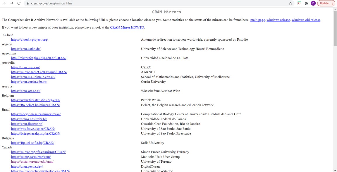
When you get here, click on the link for a mirror that is close to you. Coincidentally, being in Boston, Massachusetts, the closest to me is at the University of Toronto. Once you click on this, you should reach the following screen:

2.2.3 The R Interface
Navigate to where R was installed on your computer and open the program. Depending on how you responded to the prompts in the installer, you will probably find it in a folder titled R. You will see something that looks a lot like this:
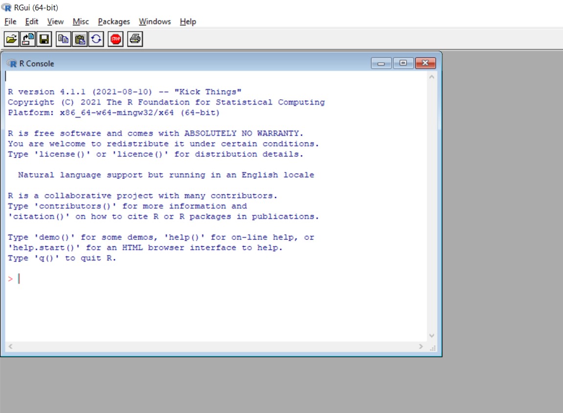
This is the R Console. You can enter code at the prompt, and R will execute that code. You can use code to import data, analyze it, and generate visualizations. There are also a few drop-down menus that facilitate certain actions by point-and-click. The default RGui (general user interface) is a bit spartan, however, with few tools available to even keep track of what you have done and created. We could really use something that is more user-friendly that combines the flexibility and control that we have through coding with some other features that make that work more efficient and its products more accessible. Luckily, such a tool exists.
2.2.4 Installing RStudio
Rather than work in the default RGui, many analysts work instead in RStudio. RStudio is known as an Integrated Development Environment (or IDE) . An IDE is software that coordinates numerous tools required to write and test software. Though it might not feel like it, every time you conduct an analysis or create graph while working with this book, you will be writing (and testing) software! An IDE is simply an interface that enhances this process, allowing you to keep track of the code you have written, the products it has generated, and the tools you are using. RStudio is not the only one built for R, but it is the best and most popular at this time.
Let us download RStudio here: https://www.rstudio.com/products/rstudio/download/. You will note that RStudio is not freeware in all cases, but there is a free version that is completely sufficient for our (and most people’s) purposes. Click DOWNLOAD under RStudio Desktop and then select the version to corresponds to your operating system.
2.2.5 The RStudio Interface
Once you have installed RStudio, navigate to it on your computer and open it. You should see something that looks like this:

There are three components visible here.
- On the left side of the screen you have the Console, which, as in the RGui, is where you can submit code directly to be executed.
- On the top right is the Environment. This is where data objects (including data sets) and some of their basic details will be listed. Behind this there are tabs for your History, or the code you have previously entered, and Connections to external sources. We will not use these often in this book.
- On the bottom right, there is a list of packages that you have installed, some of which have checks next to them, which means that they are currently enabled or “turned on.” This is also where Plots and Help will appear, as well as where you can navigate your File Directory to view the contents of your computer while in R.
We will learn more about how and when we use each of these tabs in the coming sections, but for now it is useful to know that they are there. Also, RStudio is highly customizable, so you can resize and move all of these tabs around and play with the appearance through the Tools menu, selecting Global Options.
2.3 Creating a Project in RStudio
An appealing feature of RStudio is the ability to create projects. A project is a combination of files that are all related to each other. Typically, analysts use projects to keep their work organized. Each project references a specific file directory on your computer where it stores all of its products (unless instructed to do otherwise, though we will get to that).
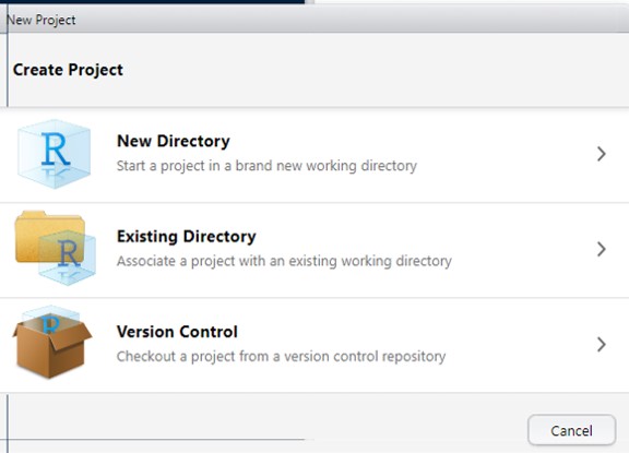
Create a new project in RStudio by clicking the File menu and then clicking “New Project…”

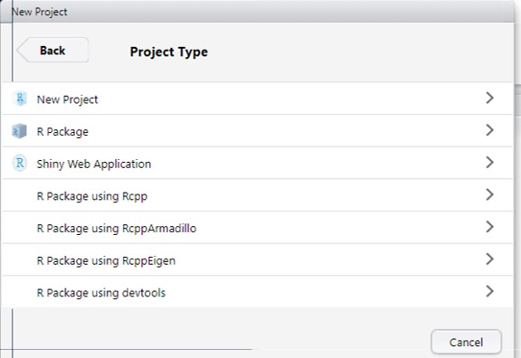
You will then be presented with this interface, where you want to select New Directory.
Then select New Project.
You will then need to specify a directory, as I have done here.
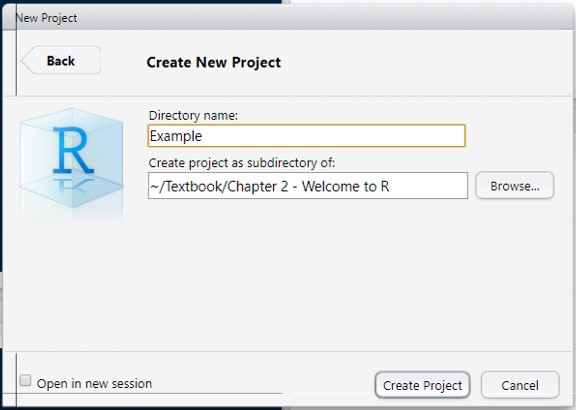
Note that you are creating a new file folder at this time that will then be the home for any files generated by the project. The folder name will also be the name of the project. (The process is slightly different when using an existing directory, but if you can do this successfully, you should have no trouble with the other.)
When you click Create, you will note that your RStudio resets. The Files tab will be on top on the bottom right now, and it will be viewing the contents of the new folder you have created. If you put files in this folder or generate products while using R, they will become visible here.
2.3.1 Creating a New Syntax
Before we get started really exploring R’s capabilities, we should have a syntax file open. As noted, we can enter commands through the Console and R will execute them. The challenge here is that this will occur line-by-line, and if we make any mistakes it is hard to go back and correct them. Instead, we want the flexibility to write multiple lines of code and to submit them to the Console in bunches. To do this, we write our code in syntax files.
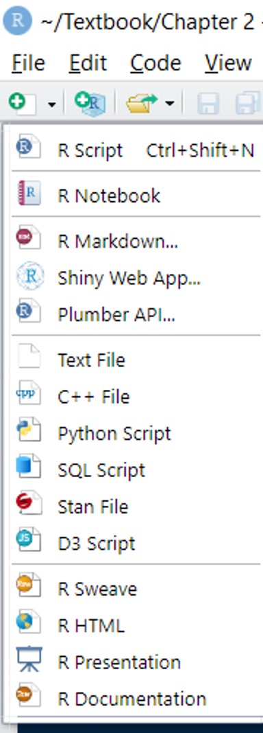
Create a syntax file by clicking this button in the upper-left-hand corner, beneath the File menu:

And then selecting R Script:
Your screen should then look something like this:

This script file is now our canvas. When we are ready to send lines of code to the console, we can select lines of code and click ctrl+Enter or tap the Run button in the top right of the script window.
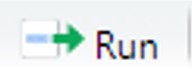
If we want to run one line of code, we can put the cursor on that line and hit ctrl+Enter, but be careful—if you do that with the Run button, it will run the entire script, which you might not want.
2.4 How to Work with R
2.4.1 Coding in R
I have mentioned a few times now that work in R is done through code. That is, an analyst must write commands that can be executed by R. This might seem daunting if you have never coded before, especially when one hearkens back to the point-and-click simplicity of Excel. Sure, there are challenges to coding. One has to know what terms the computer will recognize to do a particular job. The code has to be precise, because any typo will lead the computer to do the wrong thing or, more likely, produce an error message. This is especially important here because R is case-sensitive; meaning it interprets upper- and lower-case letters as distinct from each other. Analysts who want to do more complex tasks have to fit multiple pieces of code together to achieve that task, which further necessitates close attention to detail and often multiple tests (and failures) that require debugging.
Despite its challenges—and possibly because of them—code is also extremely useful and gives analysts complete control over their work. First, code is often a more direct pathway to accomplish a given task. For instance, in Excel it might take a half-dozen clicks to create a graph. In R, a graph can be generated in one line of code. Second, code allows the analyst to precisely specify and customize details as they go. The same graph in Excel will start with defaults—the names of the axes, the number of tick marks, even the colors of the lines or bars—that then need to be modified manually. In R, the analyst can incorporate these details into their code at the front-end. Third, code is replicable, which holds benefits for the analyst and their colleagues. Let us suppose you have written a line of code for the exact graph that you want, but you want to make this graph repeatedly for 10 variables. All you need to do is copy and paste the code, changing only the variable name. Once the initial work is done, the replication takes minimal effort. Additionally, you can share that code, plus anything you did before or after, with colleagues who can then replicate the work, refine it, or add to it.
Last, though I may be biased here, once you get the hang of it, coding is fun! You get to identify a product or outcome that you want to reach, determine the steps for getting there, and then build and execute those steps. Writing a successful sequence of code is an immensely gratifying process and not all that different from doing a crossword puzzle or solving a brainteaser.
R code is capable of supporting a lot of tasks, but at its foundation it is constructed to do two things: be a calculator and manage data. Let’s learn more about each.
2.4.2 R as Calculator
Many of R’s functions are built upon the underlying ability to operate as a calculator. Try entering the following line of code into your Console, or practice putting it in your Script and running it from there:
6+5## [1] 11R supports all traditional operations, like exponents, for example. Try:
8^2## [1] 64R is more like a scientific calculator than a basic calculator in which you have to enter one operation at a time. R can accommodate equations of any length. In doing so, it follows the order of operations rules of PEMDAS, or: solve what is inside Parentheses first, then calculate Exponents, then Multiplication and Division, then Addition and Subtraction.
For example (see if you can check R’s math):
75/25*3+15/(8-3/3+16/64*2-1264*0)-1## [1] 10This would be a good time to take a break and try a few arithmetic equations of your own, just to make sure you are comfortable.
2.4.3 Functions
This is our first opportunity to engage with functions in R. Functions are built-in commands that instruct R to complete certain calculations or tasks. Generally, functions are followed by parentheses, and the function is performed on the contents of the parentheses. In this book, functions will be formatted as R code inline.
R has many functions, including all of the ones you would expect from a calculator, including square root (sqrt) , absolute value (abs) , and trigonometric functions (e.g., sin and cos) . Others are listed in Table 2.1.
| Function | What It Calculates |
|---|---|
| abs(x) | Absolute value of x |
| cos(x) | Cosine of x |
| exp(x) | e^x |
| log(x) | Natural logarithm of x |
| sin(x) | Sine of x |
| sqrt(x) | Square root of x |
| tan(x) | Tangent of x |
Let’s try a few examples.
sqrt(100)## [1] 10abs(-25)## [1] 25We can even incorporate them into more complex equations:
sin(0)*sqrt(169)+abs(35)-cos(0)## [1] 34Before moving on, try breaking that one down into its pieces to see why that was the answer. Also, this would be a good time to take a break and try a few arithmetic equations of your own, just to make sure you are comfortable.
2.5 R as Data Management Software
R, of course, is more than just a calculator. It is an environment within which data can be managed and manipulated. As such, it is what we call an object-oriented programming language . That is, it recognizes multiple classes of objects that contain data in various forms and structures. Each class of object has characteristic features that allow R and its functions to describe and modify it. This may seem a bit abstract at this point, but what it means for our purposes is that: (1) we can store data in objects that have names; (2) functions can be applied to these objects just as if they were the numbers in the arithmetic equations we calculated in the previous section; and (3) nearly every analysis we conduct in this book will generate additional objects, meaning we can apply functions to them as well. Like functions, objects in this book will also be formatted as R code inline.
Let’s walk through the most common object classes for storing data.
2.5.1 Variables
A variable is a single value stored in an object. It might seem silly to store a single value in an object, but there are cases in which it could come in handy. For example, let us say you are looking at Boston’s open data portal and want to calculate certain records per 1,000 residents. In 2020, the population of Boston was 675,647 people. That’s a big number to have to enter repeatedly, though. What we can do instead is store it in an object that we will call bos_pop. See Table 2.2 for more on naming objects.
| Rules for naming objects… |
|---|
| 1) Must begin with a letter or dot (.). |
| 2) Can only contain letters, numbers, underscores (_), or dots (.). |
| 3) A variety of words used for programming cannot be used, including if, NA, TRUE, FALSE, else, function, and others. |
| 4) It is good practice to give objects names that help you and others to recognize what they mean when they are embedded in code. |
| 5) Keep in mind that R is case-sensitive, so you will always have to reference the object exactly as you wrote it. Also, it is possible to have multiple objects with the same name but different capitalizations, but that would be highly confusing. |
We can create a variable in two ways. The more common is arrow notation:
bos_pop<-675647
bos_pop
## [1] 675647By putting a ’<-‘ in between the name that we want to give the variable and value we want to attribute to it, we instruct R to create that variable and give it that value. Note that R does not print the variable after this step. Instead, if we want to confirm that R did this, we need to tell it to do so by typing in the name of the variable and submitting it as a separate line of code. Also, your Environment should now have the object bos_pop in it. Note that for variables, the Environment also tells us the value. Last, R uses commas for specific purposes of separating information, which is why we enter numbers greater than 1,000 without them.
The second and less common way to do this is with an equals sign:
bos_pop=675647
bos_pop
## [1] 675647Though the arrow might seem odd or uncomfortable at first, it is the more standard practice and eventually becomes natural. You might even think of it as the arrow “storing” the value in the variable. Now, to use our variable. Boston received 251,374 requests for service through 311 in 2020. How many is this per 1,000 residents?
251374/bos_pop*1000## [1] 372.0493Meanwhile, the City approved 37,460 building permits. How many is this per 1,000 residents?
36351/bos_pop*1000## [1] 53.80176And there were 70,894 crimes reported, making for
70894/bos_pop*1000## [1] 104.9276per 1,000 residents.
Suppose we had wanted to simplify our code here, we might have constructed a second variable based on the first
bos_pop_thou<-bos_pop/1000
bos_pop_thou
## [1] 675.647Here we have illustrated a numerical variable that can be incorporated into arithmetic equations. It is, of course, possible to store characters (i.e., letters and other characters) in a variable as well. We will do more with this in the next section (Section 2.5.2) on vectors. In addition, variables can store dates and logical statements (TRUE/FALSE).
2.5.2 Vectors
A vector is a collection of values of the same type (i.e., numeric, character, etc.). For example, we might want to combine our counts of 311 requests, building permits, and major crimes in a single place. We can do this with c(), which stands for combine, with commas between each value:
bos_events<-c(251374, 36351, 70894)
bos_events
## [1] 251374 36351 70894Note that bos_events is now visible in your environment as

Communicating that it is a numerical (num) vector with 3 elements ([1:3]). (In R, putting a colon in between 2 numbers indicates a range. In fact, you can use the same convention when writing code. Try the following piece of code and see what happens: range_vector<-1:3.)
Vectors can make certain tasks more efficient because calculations can be applied across all of their elements. For instance:
bos_events/bos_pop_thou## [1] 372.04931 53.80176 104.92757We have now divided all three of our counts by the population of Boston in thousands, calculating the number of events per thousand for each in one line of code. This is illustrative of vector arithmetic in general, with the operation being applied to each of the elements in the vector and the output being a new vector of the same length. We could also store this as a new object if we so choose:
bos_events_percap<-bos_events/bos_pop_thouLast, it is possible to have vectors that store character data. Before moving on, we can create one
bos_event_types<-c('311','Permits','Major Crimes')For character data, we put ’’ or “” around each value and then commas between them outside the single or double quotation marks.
Also, I have stopped printing the content of newly made objects at this point, but you are welcome to check them on your own to confirm you entered the code correctly.
2.5.3 Data Frames
Possibly the most common and useful class of object in R—and certainly the one we will use most often in this book—is the data frame. A data frame is what you might typically envision as a spreadsheet in Excel: a set of rows, or observations, and columns, or variables. In other words, each observation has a value for each variable.
In R, we can think of the columns as a series of vectors. In fact, we can construct a data frame by combining vectors with the data.frame function:
boston<-data.frame(bos_event_types,bos_events,bos_events_percap)Data frames are often too large to view easily in the console, so we can use the View() function:
View(boston)This will produce the following view in a new tab alongside your syntax:
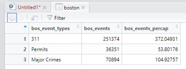
Thanks to the way we constructed our vectors, the information here is cleanly aligned, with event types matching their frequency and rate per 1,000 residents. If, however, we had a fourth row for, say, Votes Cast, but had not entered events or calculated events per capita, we would have blanks in the fourth observation. R does not do blanks, though. Instead, the value NA would be filled in, as you see here.

This is true in any R object: blanks are filled in with the value NA.
2.5.4 Other Object Classes
Variables, vectors, and data frames constitute the most basic and logical ways to organize information and they are the types of objects we will most often work with in this book. Nonetheless, there are various other classes of object that can be useful.
Lists. A list is a container for an any number of objects of any type. They may be useful in complex processes in which you want to hold a set of disparate information together for easy reference.
Matrices. Many of you may have encountered matrices in algebra classes over the years. Matrices are similar to data frames in that they have rows and columns. However, there are two major differences. First, all elements must be of the same type (e.g., numeric or character). Second, R does not treat the columns as independent vectors that can be separately named and examined.
Function-specific objects. Some functions, especially those used in statistical analyses, generate new objects. For instance, the function for running regressions, which we will learn about in Chapter 12, generates objects of the class lm for linear model. These and other function-specific objects have their own characteristic structure that allows them to be represented and analyzed in multiple ways.
2.6 Packages
R is a very powerful tool. But the functions built into R, or what we refer to as Base R, only go so far. Packages, however, use the components of Base R to enable additional tools and functions. As noted, R has a large community of users who have leveraged its opensource structure to create their own packages, each of which expands the capacities of R, creating new functions (and, in many cases, new classes of objects associated with those functions). This gives R possibly the greatest breadth of functionality of any statistical software.
R packages are published in multiple public repositories, the most prominent being CRAN. Just to give a sense of scope, there are 18,155 (!!) available packages on CRAN at the time of this writing. In fact, Joseph Rickert, an employee of RStudio, maintains a blog that reports on the “Top 40” new R packages posted every month (in his opinion). Now, of course, as with any opensource or crowdsourced effort, these packages vary in their quality—some have limited utility, mistakes that will generate frequent errors, or are just poorly constructed, but others enable the most cutting-edge tools in statistics and visualization.
We will see a variety of packages in this book, including for working with graphics (ggplot2 (Wickham et al. 2021); Chapter 3), character variables (stringr (Wickham 2019)); Chapter 4), dates (lubridate (Spinu, Grolemund, and Wickham 2021); Chapter 5), and spatial data and maps (sf (Pebesma 2021); Chapter 8), and a whole bunch for advanced visualizations (Chapter 9). Here we want to learn about and install one called tidyverse (Wickham 2021). Actually, tidyverse is not a single package but a suite of packages that have been designed to make coding in R more “tidy” by streamlining certain processes and introducing some new capacities. Don’t worry, though, you won’t have to install all these packages individually. tidyverse will install them all for you.
Enter the following code into your Syntax or Console:
install.packages('tidyverse')You will see quite a bit of activity in red—that’s R contacting a CRAN mirror site for each of the components of the tidyverse—and then some white text—that’s R unpacking and confirming that all of the packages are ready to use.
We do not have much use for tidyverse now, but we will start using it in the next chapter. Because tidyverse intends to spruce up what Base R already does for us, we can replicate pretty much every task we conduct in Base R in tidyverse. Often, the latter is more straightforward, but there are times when Base R can be preferable, if just for personal style. There is also value to understanding the underpinnings of Base R. Thus, throughout the book, we will learn everything in both ways and you are welcome to use the approach that is most comfortable for you.
That said, we might as well activate tidyverse now, just to get in the practice. When we install packages, they are not automatically loaded into an R session. This is to avoid swamping your computer’s memory with lots of extraneous tools. To activate a package we need to use either the require() or library() function (they do the same thing). Try it now:
require(tidyverse)2.7 Learning R
As we move on to more serious material in the next chapter, keep in mind that part of the goal of this book is not so much to teach R but to teach you how to learn R. This is an important distinction. This book will teach you numerous packages, functions, and techniques in R. But no textbook can communicate all of what R can do, nor would that be a practical endeavor. Likewise, analysts have not memorized every function available in R. We all have to reference documentation from time to time, either to recall how to use old functions and packages or to find new ones. There are two tricks that come in handy.
Help. RStudio has a tab for Help that is in the bottom-right viewer by default. This searches and browses the detailed documentation available for all functions and packages. You can use ? in the console to bring up the documentation for any function or package. (Try, for example, ?sqrt.) You can also access these documentations from CRAN.
Google. It sounds silly to say, but an important tool for learning any coding language is Google. This is especially true when you are trying to solve a problem but do not yet know what functions or packages you should be using. In such cases the help documentation is not as helpful. But if you Google your problem, it is very possible someone else has encountered or solved the same issue. It is just a matter of entering a set of search terms that will be similar to the terms those who came before you might have used to describe the problem or the tool you need for it.
2.8 Summary
In this chapter, we have:
- Installed R from one of the mirror sites available at https://cran.r-project.org/mirrors.html;
- Installed RStudio from https://www.rstudio.com/products/rstudio/download/.
- Become familiar with the RStudio interface, including:
- Creating a new project,
- The Console, where data are submitted and results reported,
- The Environment, where objects in your project are visible,
- Creating a new Script for building code.
- Used R as a calculator that can execute arithmetic equations.
- Used R as a data management software that can store, manipulate, and examine:
- Variables, or single values;
- Vectors, or collections of values of a single type;
- and Data Frames, or sets of observations (rows) with values on each of two or more variables (columns).
- Accessed packages, specifically those composing
tidyverse, which expand the capabilities of R. - Learned how to learn R by using Help and Google.
2.9 Exercises
2.9.1 Problem Set
- In the next chapter we will learn a variety of new functions. Learn a bit about them now by using ?. Describe in your own words what each does.
?nrow?length?nchar?read.csv
- Classify each of the following statements as describing a variable, vector, data frame, two of them, or all three.
- Can only contain one type of data (e.g., numeric, character).
- Consists of multiple values.
- Consists of multiple vectors.
- Can be given any name starting with a letter.
- Define each of the following terms and their importance for analysis with R:
- Object-oriented programming
- Function
- CRAN
2.9.2 Exploratory Data Assignment
Just as we did in this chapter, create a new data frame from a series of vectors. Before you start, map out the elements.
- What are the observations?
- What will the variables be that describe them?
- Generate a
Viewof the final product (take a screenshot) and describe the contents in no more than a paragraph or two.