7 Making Measures from Records: Aggregating and Merging Data
Allegheny County, the home of Pittsburgh, Pennsylvania, had a problem with truancy. This is not an uncommon situation. A lot of urban areas have large populations of at-risk youth who are regularly absent from school. The County also recognized an institutional challenge to fixing the problem: the people responsible for supporting these youths were case workers, but case workers did not have access to school attendance records because they worked for the Department of Human Services (DHS), not the school district. To make things even more complicated, DHS was run at the county level and schools were run by each of Allegheny County’s 43 school districts. Thus, case workers were not aware of when one of their cases was missing school. What to do?
Enter Erin Dalton, director of Allegheny County’s Data Warehouse (and later Director of all of Health and Human Services). The Data Warehouse is an example of an Integrated Data System (IDS) that merges data from across the many Health and Human Services departments in a government for each individual. Through the Data Warehouse, Erin’s team was able to link a case worker’s profile with data on each of the kids they worked with from the appropriate school district. They were even able to do updates in real-time and created an alert system so that a case worker was notified if any of those children were absent for three consecutive days.
An IDS is a powerful infrastructure that takes advantage of the many different ways that people interact with government services. As Erin likes to quip, if the mayor (or county chair, in this case) has to sign both sides of a data-sharing agreement, you don’t need a data agreement. Data-driven departments in over 35 states, counties, and cities have embraced this perspective (see Figure 7.1), enabling a variety of innovative approaches to practice, at least according to Actionable Intelligence for Social Policy, a national consortium of IDSes based at the University of Pennsylvania.
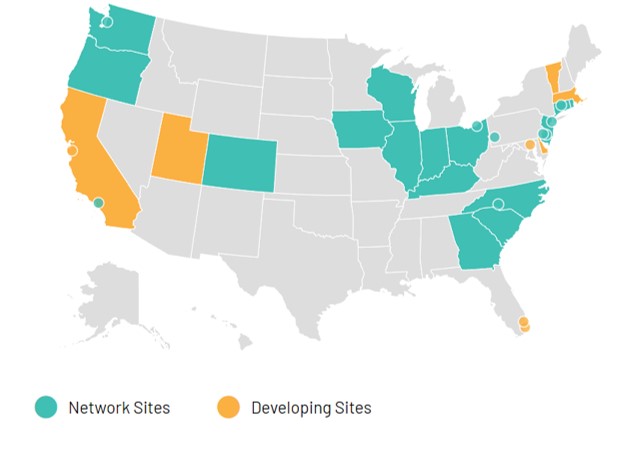
Figure 7.1: A map of the states, cities, and counties that are members of Actionable Intelligence for Social Policy, a network of IDSes. (Credit: Actionable Intelligence for Social Policy).
Let us consider for a moment how IDSes operate from a technical perspective. They are premised on the tools we discussed conceptually in the previous chapter. They first must create measures for individuals in the system by aggregating all records from a given data set referencing that individual. This is possible for any data set, whether it is generated by a hospital, human services, school districts, the criminal justice system, homelessness services, or otherwise. They can then merge these measures using unique identifiers (or key variables) made available by the schema (i.e., name, social security number, birthday, etc.). The technical process of aggregation and merger is the focus of this chapter.
7.1 Worked Example and Learning Objectives
In this chapter, we will take the next step with the two tools fundamental to IDSes—aggregating and merging data sets—by learning the technical skills necessary to execute them. Of course, working with detailed human services data can require specialized access for privacy reasons. As such, in this chapter we are going to work through the original human services data: census data. And to illustrate how it can work at its most granular level, we will use census data for Boston from 1880, which is old enough that the raw data have been released: the gender, ethnicity, profession, and more are included for every individual. Working with these data we will learn to:
- Create aggregate measures in base R and
tidyverse; - Merge data sets on shared key variables in base R and
tidyverse; - Use SQL, another coding language common to database management that can be utilized in R through the
sqldfpackage, to aggregate; - Create bivariate (i.e., two-variable) visualizations in
ggplot2, including dot plots.
Link: https://dataverse.harvard.edu/dataset.xhtml?persistentId=doi:10.7910/DVN/28677. You may also want to familiarize yourself with the data documentation posted there.
Data frame name: census_1880
Note: The data set contains census records from 1880-1930. We will limit the data to 1880 from the outset.
hist_census<-read.csv('Unit 2 - Measurement/Chapter 07 - Aggregation and Combining Data/Example/Census Data 1880_1930.csv')
names(hist_census)[1]<-'year'
census_1880<-hist_census[hist_census$year==1880,]
7.2 Aggregating and Merging Data: How and Why?
Working with records is both challenging and empowering for an analyst. They are challenging because a record may reference one or more traditional units of analysis—a person, place, or thing—but it does not fully encapsulate that unit of analysis. A discrete unit might be referenced by 1, 10, 30, 100, or zero records. Often we are not interested in analyzing the records themselves but the units of analysis that they reference.
At the same time, records can be empowering. Their composite describes the desired units of analysis in highly nuanced, detailed ways. One might leverage a set of records to generate dozens of descriptors for those units of analysis. How many records for each individual unit appear in the data? What types of records? If the records have quantitative values associated with them, we can calculate the mean, the sum, the min, the max, or other statistical features of those values for each individual unit. This flexibility empowers the analyst to generate the precise measures needed to describe the objects of interest.
The key to going from records to units of analysis is aggregation, or the gathering of information at one level of organization to describe a higher one. For example, from records to people, or from people to neighborhoods, or from neighborhoods to cities, and so on. The other key tool here is merging, or the linkage of data sets on shared key variables. We can create aggregate measures for the same unit of analysis from multiple data sources and then link them by unique identifiers, or one or more variables that distinguish each unit in a set of units. And this is all made possible by a schema, or the organizational blueprint of how a data set’s structure relates to other data sets at various levels of analysis.
7.3 Introducing the Schema for Historical Census Data
Before we get started, let’s acquaint ourselves with the schema of the historical census data. Admittedly, we only have one data set, whereas a typical schema consists of multiple interlocking data sets at different units of analysis. Nonetheless, the census data does reference numerous nested units of analysis, making for a simple but illustrative schema for us to learn from.
By using the names() command we can take a look at the contents of the historical census data more closely. You might also want to download the data documentation and take a direct View() of the data as well. Each row is an individual with a variety of descriptors, including their gender, age, profession, and heritage (e.g., native-born vs. immigrant). There is also a series of variables that describe the broader organization of the data set and how it links to other units of analysis.
At the front end of the data set, we have the variable serial, which is a unique indicator for the household. Note that there are many cases in which multiple rows share the same value for serial, reflecting the fact that the data is a list of all individuals organized by household. There is also the variable pernum, which itemizes the individuals in each household (e.g., if there are two members of the household, they have the values 1 and 2). There are also enumeration districts (enumdist), or the rather small regions that the census used for organizing the geography of the city. Households (serial) are nested in enumeration districts. Further, enumeration districts are nested in census wards (ward), somewhat larger administrative regions. If we were working with data from across the country, we would also have wards nested in multiple cities (city). Instead, we just have all the wards that constitute Boston.
The historical census provides us with an ideal opportunity to aggregate data. We have individuals nested in households, households nested in enumeration districts, and enumeration districts nested in wards. We can aggregate up from our records to any of these other levels. (It is also worth comparing this structure with the example schema of the modern Geographical Infrastructure described briefly in Chapter 6. They are very similar!) If we happened to have outside data on any of these other levels—say, voting results for wards—we could link that information in as well. Here we will focus mainly on individuals, households, and wards.
7.4 Aggregation
Aggregation is the process of using cases from one unit of analysis to describe a higher order unit of analysis. Examples include using discrete credit card transactions to describe the purchasing patterns of individuals, using household characteristics to describe the demographics of a community, or using counts of 311 or 911 reports to measure disorder and crime on a street. Aggregation depends on three pieces of information: (1) the unit of analysis for the initial data set, (2) the unit of analysis to which we want to aggregate, and (3) the function by which we want to aggregate (e.g., the count of cases, the sum or mean of case values, etc.).
We have already learned the most basic way to aggregate, which is to use the table() command to generate counts for all values of a variable. For instance, to calculate the number of individuals in each household, we could do the following, using code originally seen in Chapter 4.
hh_people<-data.frame(table(census_1880$serial))
head(hh_people)
## Var1 Freq
## 1 483155 2
## 2 483156 5
## 3 483157 6
## 4 483158 4
## 5 483159 6
## 6 483160 2If you View() the result you will see a list of all households and the number of people living there. This technique is a little clunky, as the variable names (Var1 and Freq) are artifacts of using the table() command. It also is limited to counts. In this section we will learn the commands that are designed to flexibly conduct all types of aggregations in base R and tidyverse.
7.4.1 aggregate()
In base R the primary command for creating aggregations is, fittingly, aggregate(). The aggregate() command can be specified in a number of ways, but its simplest form is aggregate(x~y, data=df, FUN) where data= indicates the data frame we want to aggregate from, y is the unit of analysis to which we want to aggregate, x is the variable we want to use to describe that level of analysis, and FUN is the function we will apply to x. The ~ symbol—which we also saw in Chapter 5 when learning how to make facet graphs—is used in R to indicate one variable (x) being analyzed as a function of another variable (y). We will encounter it with some frequency from here on, especially in Part III.
Let us begin by replicating the example we did above with the table() command. Oddly, base R does not have a good function for counting things. There are a couple of workarounds, one of which is to use tidyverse, as we will see in Section 7.4.2. For now, the historical census data offer us another option because it has already counted out the number of individuals in each household with the pernum variable. Thus we can take the maximum value on this variable for each household (serial).
hh_people2<-aggregate(pernum~serial, data=census_1880, max)
head(hh_people2)
## serial pernum
## 1 483155 2
## 2 483156 5
## 3 483157 6
## 4 483158 4
## 5 483159 6
## 6 483160 2If you compare this product side-by-side with hh_people, which we created using the table() command, you will note that they are identical except the variables are a bit more explanatory (serial and pernum).
What else might we do? We could use the age variable to calculate the oldest person in the house. Before we do so, let us take a quick look at this variable.
summary(census_1880$age)## Length Class Mode
## 37209 character characterWe seem to have a problem. R thinks that this variable is a character variable. We need to fix this (if the following lines of code seem odd, check out table(census_1880$age) to get a sense of how (and why) we are modifying the variable).
census_1880$age<-ifelse(census_1880$age=='90 (90+ in 1980 and 1990)','90',as.character(census_1880$age))
census_1880$age<-ifelse(census_1880$age=='Less than 1 year old','0',as.character(census_1880$age))
census_1880$age<-as.numeric(census_1880$age)
Now that we have replaced the text values with numerical ones and then converted the class of the variable to numeric, let’s try again.
hh_oldest<-aggregate(age~serial,data=census_1880,max)
table(hh_oldest$age)
##
## 5 6 7 8 9 10 11 12 13 14 15 16 17 18 19 20
## 5 6 7 10 16 25 19 24 19 23 26 23 16 26 30 25
## 21 22 23 24 25 26 27 28 29 30 31 32 33 34 35 36
## 36 46 64 48 122 107 114 135 148 250 134 176 139 159 340 185
## 37 38 39 40 41 42 43 44 45 46 47 48 49 50 51 52
## 166 240 176 514 102 189 154 134 390 136 128 172 112 464 81 152
## 53 54 55 56 57 58 59 60 61 62 63 64 65 66 67 68
## 115 128 233 140 87 109 78 332 67 101 97 85 182 66 74 78
## 69 70 71 72 73 74 75 76 77 78 79 80 81 82 83 84
## 57 174 40 48 50 51 55 35 26 30 27 56 14 18 13 12
## 85 86 87 88 89 90 91 92 94 96 98 99 103 108
## 9 4 12 8 4 9 5 4 1 1 3 2 1 1The table here is far more intelligible, ordered numerically rather than textually. The most common age for the oldest member of a household is now 40 (514 households). There are still some odd cases of minors being the oldest member of the household, but far fewer. This may tell us something about the completeness of the census data, the way households were defined for orphans, or typographical errors. We are not going to probe this oddity any further, however. That said, if we want to, we can now use similar code to calculate the youngest person for each household.
hh_youngest<-aggregate(age~serial,data=census_1880,min)7.4.1.1 aggregate() with a Logical Statement
There are a variety of extensions of the use of aggregate() we might pursue. The first is to use a logical statement. Suppose we want to know how many minors are living in a house. We first need to define ‘minor’ in our records as individuals younger than 19, or hh_youngest$age<19.
We can incorporate this statement into an aggregate command, like so
hh_children<-aggregate(age<19~serial,data=census_1880,sum)Our logical command has created a dichotomous variable based on whether age is less than 19, and then summed over this variable for every household. Minors are equal to 1 and adults are equal to 0 on this variable, so summing effectively counts the number of minors. If you look at the names of the resulting data frame, however, you will see that the second variable has an odd name because it is drawn from the logical statement.
names(hh_children)## [1] "serial" "age < 19"We will need to fix this.
names(hh_children)[2]<-'children'We might do something similar for immigration status. Looking at the codebook, any value greater than 2 on Nativity indicates a person who immigrated to the United States.
hh_immigrant<-aggregate(Nativity>2~serial,data=census_1880,max)
names(hh_immigrant)[2]<-'immigrant'
By using the maximum function, we have now determined whether each household has at least one immigrant living there (i.e., the maximum of the dichotomous variable of whether each resident is an immigrant or not; if anyone is an immigrant, the maximum is 1, otherwise it is 0).
7.4.1.2 aggregate() Multiple Variables at Once
You may have noticed that we are creating a new data frame each time we run an aggregation. We can bring them together later with merging. Even more inefficient, however, is that we have used the same function on multiple variables. We could instead apply the same logic of aggregation to multiple variables using the cbind() command, which stands for “column bind,” or connecting multiple columns together.
hh_maxes<-aggregate(cbind(pernum, age)~serial,
                    data=census_1880,max)
head(hh_maxes)
## serial pernum age
## 1 483155 2 55
## 2 483156 5 42
## 3 483157 6 41
## 4 483158 4 65
## 5 483159 6 50
## 6 483160 2 22This command creates a data frame with three columns: serial, pernum as the number of people living in each household (i.e., the maximum value for pernum), and age as the age of the oldest person in the household. Importantly, we have to use cbind() for this, not c(). If we used c() it would combine all values from the two columns into a single list that would be twice the length of the list of households (serial). This would generate an error (go try!).
7.4.1.3 aggregate() with Two Grouping Variables
Suppose we want to create an aggregation based on two different variables. In past chapters, for example, we might have wanted to aggregate on the combination of month and year, or day of the week and month. Here, we might want to keep the information about the ward as we aggregate from the individual to the household. We then need both variables in our aggregate() command. This takes the following form:
hh_people<-aggregate(pernum~serial+ward,data=census_1880,max)
head(hh_people)
## serial ward pernum
## 1 483155 1 2
## 2 483156 1 5
## 3 483157 1 6
## 4 483158 1 4
## 5 483159 1 6
## 6 483160 1 2We now have a new data frame with three variables (note that if you are following the code faithfully, we have overwritten the previous hh_people that we created with table() earlier): serial, the ward of each household, and the number of people living there. This works because ~ indicates that one variable is being treated as a function of one or more other variables. Thus, the function applied to pernum is now organized by serial and ward, meaning across all of their intersections. This is something of a trivial case because households are nested in wards, meaning each serial value only shares rows with one ward value. A month-year example would be somewhat more complicated as each month occurs in each year, and the product would be the series of all months across multiple years of data.
7.4.2 Aggregation with tidyverse
Aggregation can also be done in tidyverse using the combination of the group_by() and summarise() functions, which we have already encountered in Chapter 4. These must be combined through piping. group_by() instructs R to organize any subsequent analyses by a variable (e.g., serial) and summarise() then creates variables according to specified equations. If we used the summarise() command without group_by() we would generate one or more measures describing the entire data set. With group_by(), however, we generate each of those measures for all values of the grouping variable. (Remember that you will need to require(tidyverse) to proceed with the worked example.)
Let us replicate our first aggregation, which was to count the number of people in a household using pernum.
hh_people<-aggregate(pernum~serial,data=census_1880,max)
In tidyverse, this becomes
hh_people<-census_1880 %>%
  group_by(serial) %>%
  summarise(fam_size=max(pernum))
We first indicate the initial data frame (census_1880) and then group_by() the variable serial and summarise() based on the equation max(pernum). The result is the same, though with the added benefit of being able to name our variable in advance (fam_size). Recall, however, that I said that tidyverse makes it easier for us to do counts of cases. This is the purpose of the n() function.
hh_people<-census_1880 %>%
  group_by(serial) %>%
  summarise(fam_size=n())
The group_by() and summarise() approach can easily be extended to each of the examples conducted above with aggregate() and more.
7.4.2.1 group_by() + summarise() with a Logical Statement
Above we tabulated the number of children in each household and the presence or absence of immigrants in each household by incorporating logical statements into our aggregate() commands. We can do the same by using the logical statements in the summarise() command.
hh_children<-aggregate(age<19~serial,data=census_1880,sum)
becomes
hh_children<-census_1880 %>%
  group_by(serial) %>%
  summarise(children=sum(age<19))
7.4.2.2 group_by() + summarise() Multiple Variables at Once
We can also calculate multiple variables at once with the summarise() command. What was once
hh_maxes<-aggregate(cbind(pernum, age)~serial,data=census_1880,max)
is now
hh_maxes<-census_1880 %>%
  group_by(serial) %>%
  summarise(fam_size=max(pernum), age_oldest=max(age))
But why stop there? summarise() is not constrained by a single function. We can calculate as many equations as we want at once, bringing together everything we have done so far:
hh_features<-census_1880 %>%
  group_by(serial) %>%
  summarise(fam_size=n(),
            age_oldest=max(age),
            age_youngest=min(age),
            children=sum(age<19),
            immigrant=max(Nativity>2))
Take a look at the output data frame to see what we have created.
7.4.2.3 group_by() + summarise() with Two Grouping Variables
The last thing we did with aggregate() was to have multiple grouping variables, thereby conducting the aggregation over all of their intersections. The same can be accomplished by adding variables to the group_by() command, as in:
hh_people<-census_1880 %>%
  group_by(serial,ward) %>%
  summarise(fam_size=n())
We could even combine everything we have done to this point with the following:
hh_features<-census_1880 %>%
  group_by(serial, ward) %>%
  summarise(fam_size=n(),
            age_oldest=max(age),
            age_youngest=min(age),
            children=sum(age<19),
            immigrant=max(Nativity>2))
And with that one multi-part command, we now have created a single data frame that contains the list of all households (serial) and the number of people living there, the ages of the oldest and youngest residents, the number of children, and whether any residents are immigrants, as well as the ward containing the household.
7.5 Merging
Merging data sets on key variables is often an important complement to aggregation. During the early stages of this analysis, we generated data frame after data frame, each with the serial variable and one other descriptor. Of course, the flexibility of tidyverse allowed us to overcome this inefficiency, but that was only possible because we were aggregating from a single data set. If, as in the case of an IDS, we had been working with multiple data sources to generate a variety of descriptors of households, they would have necessarily sat apart. But because they all described households, they would (at least in a well-constructed schema) share the same key variable. We can use such key variables to merge data set together to combine all variables in a single data frame.
7.5.1 merge()
Conveniently, the primary command for merging data sets in base R is merge(), which requires us to specify two data frames and the variable by which they will be linked. For example:
households<-merge(hh_people,hh_children,by='serial')
names(households)
## [1] "serial" "ward" "fam_size" "children"This merges hh_people and hh_children using the key variable serial. Thus, as we see, every value of serial will now have all variables from hh_people and hh_children side-by-side.
One limitation of merge() is that it can only handle two data frames at a time. If you have three or more data frames, you need to merge them iteratively. Let’s bring in the immigrant status variable next.
households2<-merge(households,hh_immigrant,by='serial')Something funny happened here, though, as we can see with the nrow() command.
nrow(households)## [1] 8555nrow(households2)## [1] 8544We somehow dropped from 8,555 cases to 8,544 cases. Why? It appears that hh_immigrant had 11 missing cases. If we dig further, there were 130 NAs in the Nativity variable, which means that those 11 missing households likely had NA records.
merge() has the default of only keeping rows present in each data frame. We can override this using the all= argument. In this case, we want to keep every row in the x data frame, or the first one we specified, so we use the all.x= version of the argument and set it equal to TRUE.
households<-merge(households,hh_immigrant,by='serial',all.x=TRUE)Depending on our goals, we can keep all rows in the y data frame, or the second one we specified (all.y = TRUE), or keep all rows in both data frames (all.x.y = TRUE).
Because merge() is sensitive to the particular composition of a data set and its values, there are a few other cautions and considerations that should be taken whenever merging. First, make sure that there are no duplicates on your key variables. If there are, the merge will keep these duplicates. If there are duplicates in both data frames, the final data frame will not only keep them but create new rows for all possible combinations (e.g., 3 duplicates of a single value in each data frame would generate 3*3 = 9 rows in the final data frame). With a large data set this can create an explosion of rows.
Second, R cannot handle duplicate variables. The command is designed to not duplicate the key variable in the final data frame, but it has to deal with any other variables repeated in both data sets in another way. It does so by adding the suffixes .x and .y. This can create issues with downstream code if you assume that all variable names remained the same.
Third, it is possible to merge data frames that have shared key variables but with different names. For instance, if we had renamed the variable serial to be household in one of our data frames, we could have still merged it with other data frames by specifying by.x = ‘serial’ and by.y = ‘household’. In such situations, though, make sure that you are confident that the variables really are the same, or the merge will either not find any matches or run into the issue of duplication as noted above.
Fourth, it is also possible to merge on more than one key variable. This can come in especially handy if you have aggregated on multiple variables, as we did with serial and ward. This can be accomplished using by = c(‘serial’,’ward’).
7.5.2 join functions in tidyverse
tidyverse offers the family of join functions as an analog to merge(). There is in fact no join function, but multiple functions with different names that correspond to the various settings of the all argument.
inner_join()reflects the default merge(), keeping only rows that occur in each data frame.left_join()corresponds to the all.x variant of merge(), keeping all rows in the first data frame specified.right_join()corresponds to the all.y variant of merge(), keeping all rows in the second data frame specified.outer_join()corresponds to the all.x.y variant of merge(), keeping all rows in both data frames.
In each case, the required arguments are the two data frames and the key variable. (join functions, like merge(), cannot handle more than one data frame at a time, in part because it would be logically difficult if not impossible to specify which rows to keep if each of three or more data frames had different sets of rows.) Thus,
households<-merge(hh_people,hh_children,by='serial')
becomes
households<-inner_join(hh_people,hh_children,by='serial')
and
households2<-merge(households,hh_immigrant,by.x='serial')
becomes
households2<-left_join(households,hh_immigrant,by='serial')
As you can see, merge() and the join family of commands are nearly identical and there are few if any objective advantages to one over the other. As such, it is simply a matter of preference and whether you tend to more easily remember the logic of the all argument or the different members of the join family of functions.
7.6 SQL and the sqldf Package
SQL is one of the most common softwares used for database management. Recall from the discussion of schemas that a database is consists of multiple interlocking data sets, also referred to in database terminology as “tables.” SQL is a rather simple, elegant coding language used to “query” a database and extract the desired cases. This is because databases are often constructed to store very large amounts of data that you would not want to work with in their entirety—this was especially true decades ago when databases were first invented and hard drives were measured in megabytes instead of gigabytes.
SQL has been incorporated into R with the sqldf package (Grothendieck 2017). A SQL statement is very simple, requiring only three components: select indicates the variables that you want; from indicates the table (or, in our case, data frame) you are drawing them from; and where articulates any criteria for the rows you want (like a subset in base R or filter() in tidyverse; technically, where is optional if you do not want to set any criteria). Importantly, there are no commas between commands, only between elements within commands (e.g., between multiple variables specified in the select command). We are going to learn these basic elements of SQL as well as a fourth (but optional) component of a SQL command that makes it possible to create aggregations: group by.
The main advantage of working with SQL to aggregate data rather than aggregate() is the ability to create multiple measures with different functions at once. However, with the advent of tidyverse, this is no longer as distinctive. I include it here, though, because it provides an excuse to introduce you to a skill that you might develop further if you want to go into database management at some point.
7.6.1 Aggregation with SQL
We will use SQL to illustrate a second level of aggregation from households to wards. To do so we will work from the hh_features data frame that we created in our last and most complete aggregation in the tidyverse. Before we can do that, though, we need to recode our integer variables to numeric variables because sqldf cannot handle integer variables.
hh_features$immigrant<-as.numeric(hh_features$immigrant)
hh_features$fam_size<-as.numeric(hh_features$fam_size)
hh_features$children<-as.numeric(hh_features$children)
sqldf uses a single command, sqldf(), into which a full SQL command as entered as text bounded by single quotation marks. To get started, let us first see how a simple SQL command works. We might, for example, want to look quickly at a list of only household serial numbers and their wards.
require(sqldf)
options(scipen=100)
head(sqldf("select ward, serial
             from hh_features
             "))
## ward serial
## 1 1 483155
## 2 1 483156
## 3 1 483157
## 4 1 483158
## 5 1 483159
## 6 1 483160Note that we have entered this without storing it in a new data frame.
We could also look at all variables for a single ward:
head(sqldf("select *
             from hh_features
             where ward = 5
             "))
## serial ward fam_size age_oldest age_youngest children
## 1 484456 5 4 51 1 1
## 2 484457 5 3 46 10 1
## 3 484458 5 5 61 12 1
## 4 484459 5 5 68 25 0
## 5 484460 5 3 53 9 1
## 6 484461 5 4 41 3 2
## immigrant
## 1 0
## 2 1
## 3 0
## 4 1
## 5 1
## 6 0Note that entering * after select chooses all variables, in this case for all households in ward 5.
Now we are ready to use SQL to create an aggregation. Instead of printing out the result we will now create a new data frame containing all of the aggregations for our wards.
wards<-sqldf("select ward,
             sum(fam_size) as population,
             count(serial) as households,
             sum(immigrant)/count(immigrant) as prop_imm_hh,
             sum(fam_size)/count(fam_size) as avg_hh_size,
             sum(children)/count(children) as children_per_hh
             from hh_features
             where immigrant != 'NA'
             group by ward")
Let’s break this down. First, we selected ward followed by a series of newly calculated variables. This highlights two special features of SQL: (1) you can calculate new variables on the fly, whether for aggregations or otherwise; and (2) you can name them flexibly using as. Thus, sum(fam_size) as population is identical to summarise(population=sum(fam_size)) in tidyverse. Also, SQL, unlike base R, has a count() function we can call upon for counting. We have thus calculated for each ward: the total population; the number of households; the proportion of households with at least one immigrant resident (prop_imm_hh) as the sum of our dichotomous immigrant variable divided by all households (calculated with count()); the average household size (avg_hh_size), again calculated with a sum() divided by a count() because SQL has no internal command for calculating means; and the average number of children per household (children_per_hh). If you are feeling up to it, see if you can replicate these equations in tidyverse.
After select-ing all of our variables, we had to indicate that we were generating them from the hh_features data frame. We also limited to cases in which immigrant was not equal to NA, as this would have created issues for SQL. We then grouped the newly calculated variables (group by) by ward. Importantly, I have taken a lazy shortcut here for the sake of illustration. It is, of course, necessary to remove households with no clear immigration status if we are calculating variables related to immigration status; this is indeed the purpose of na.rm = in most statistical functions. However, there is no reason we need to drop these 11 households when calculating things like average household size or average number of children. We have done so here only because it is far more efficient to demonstrate the tool in one fell swoop rather than rerun multiple aggregations. That said, you are welcome to do this the right way on your own.
7.6.2 Merging with SQL
SQL is a comprehensive language for managing the tables contained in one or more databases. It of course can do much more than just select variables and rows and aggregate them. One of its other capacities is merging. However, merging in SQL is a little bit more complicated than in R, and sqldf does not support it. We will pause in our learning of sqldf here, but there are plenty of resources for going further if you would like to do so.
7.7 Creating Custom Functions
As described numerous times, R’s flexibility and open-source nature allow analysts to easily develop new functionality and packages. We have not yet discussed how this is done, however. The fundamental building block of development in R is the creation of custom functions, and it is quite straightforward. This can come in quite handy when generating aggregations because they depend on the precise function that we want to apply to our records to then describe the higher unit of analysis.
We can illustrate by creating a function for identifying the mode of the distribution (i.e., the most common value). Interestingly, R does not have a function for this despite it being commonplace in statistics. We can create such a function ourselves.
mode <- function(x) {
  ux <- unique(x)
  ux[which.max(tabulate(match(x, ux)))]
}
We have now made an object (you can see it in your Environment) called mode. That object is a function as defined in the two lines of code contained in {}. function(x) indicates that we are creating a function that operates on a single input, x. The function itself then creates a temporary vector, ux, that is a list of all unique values in x. The following line tabulates the number of matches between x and each value in ux and selects the value with the most such matches (which.max()), which is the functional definition of a mode.
Let’s see how it works in practice. In the historical census data, birthplace is recorded for each individual. It might be interesting to know what the most common birthplace is for each household and see how it is distributed across the city.
hh_mode_bpl<-aggregate(bpl~serial,data=census_1880,mode)

data.frame(table(hh_mode_bpl$bpl)) %>%
  arrange(desc(Freq)) %>%
  head()
## Var1 Freq
## 1 Massachusetts 4636
## 2 Ireland 1496
## 3 Maine 517
## 4 Canada 454
## 5 New Hampshire 251
## 6 England 207A quick look at the values across households reveals that for the majority the most common birthplace of household members is Massachusetts, but that for nearly 20% the most common birthplace is Ireland. This is then followed by Maine, Canada, New Hampshire, and England. This is consistent with the large influx of Irish immigrants to Boston in the second half of the 19th century.
7.8 Bivariate Visualizations
We now have a data frame with a series of numerical variables describing the population of each of Boston’s wards in 1880. This makes for a convenient excuse to expand our knowledge of visualization in ggplot2 to work with bivariate plots. We have featured more than one variable in a graph previously, but it has always involved categorical variables that split up a univariate graph in one way or another (e.g., stacked or faceted histograms). For the first time we will work with the full variation of multiple numerical variables with the geom_point() and geom_density2d() commands.
7.8.1 geom_point()
Recall that our data frame of wards contains population, number of households, average household size, average number of children, and proportion of households with immigrant residents. We can examine the association of any two of these variables with a dot plot, created with the geom_point() command. For example, does the number of children per household increase with average household size? First we establish our base ggplot() command.
size_w_child<-ggplot(wards,
              aes(x=children_per_hh, y=avg_hh_size))
and then we can add on the geom_point() command.
size_w_child+geom_point()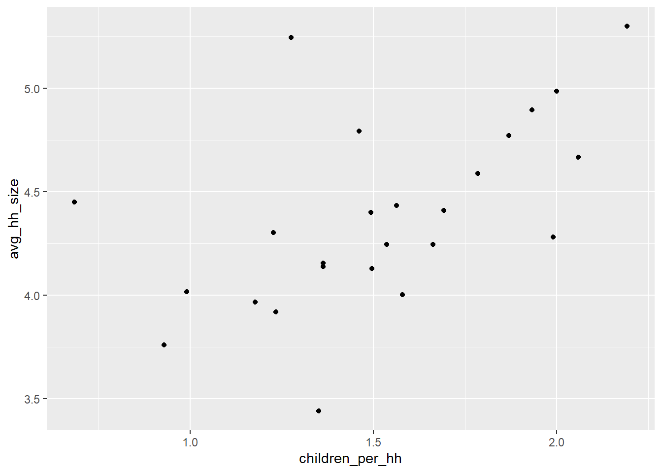
Unsurprisingly, there is a very strong correlation. As a community’s households have more children on average, the average household size goes up. There are a few outliers that violate this relationship, likely because of different norms of how many adults live together (or can afford not to). Of course, we can use ggplot’s broad functionality to make this a little prettier.
size_w_child+geom_point(colour = 'blue', shape = 0, size = 5) +
  labs(x='Children per Household',y='Avg. Family Size')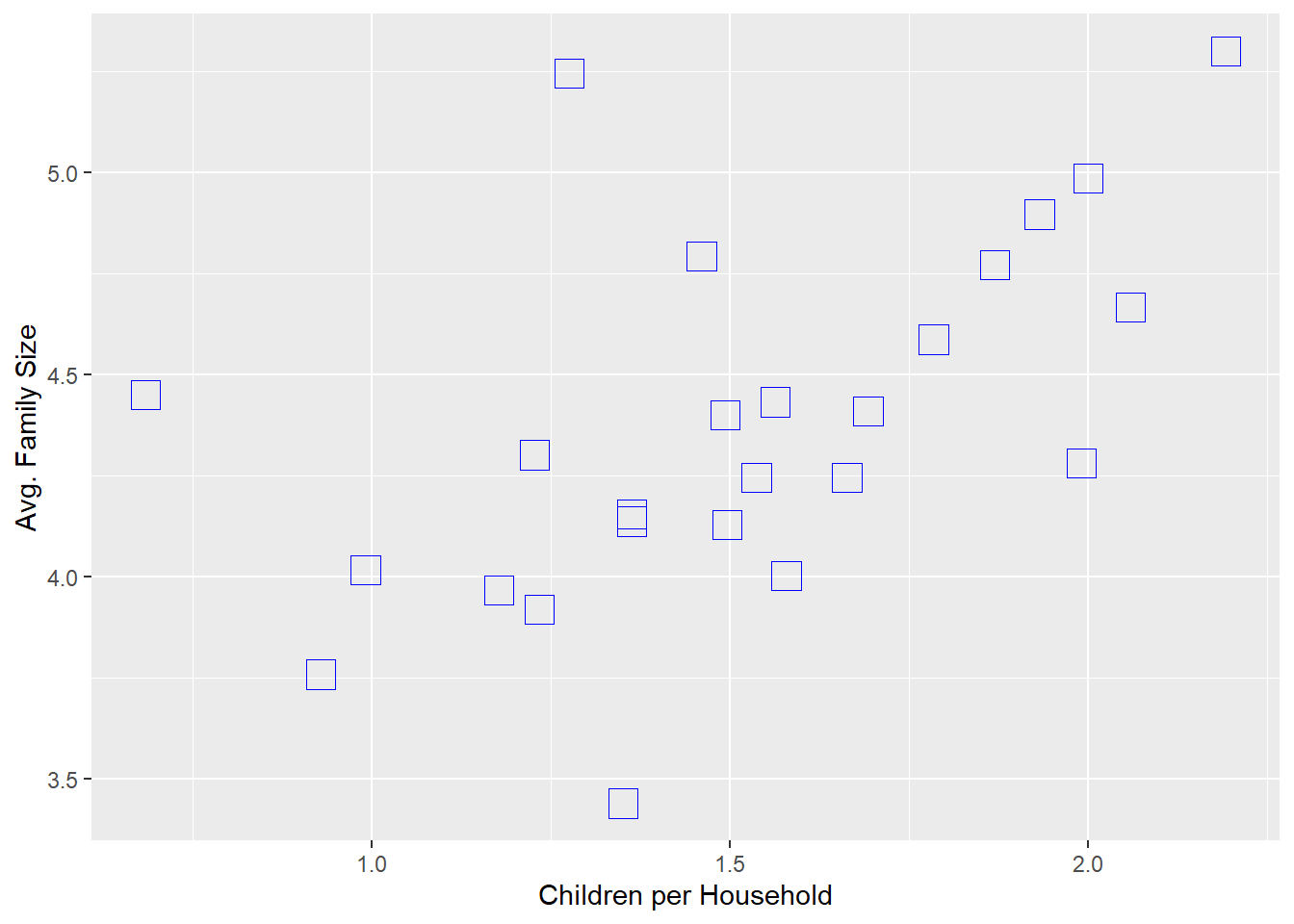
Possibly more interesting would be whether communities with more immigrant households have more children on average, suggesting that immigrant households tended to have more children in 1880 Boston.
child_by_imm<-ggplot(wards,
              aes(x=prop_imm_hh, y=children_per_hh))
child_by_imm+geom_point(color = 'blue', shape = 0, size = 5) +
  labs(x='Proportion of Immigrant Households',
  y='Children per Household')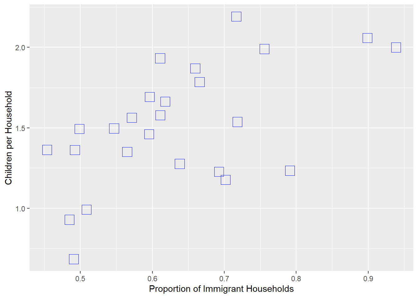
Again, we see a substantial correlation, suggesting that immigrant households tended to have more children than non-immigrant households.
7.8.2 geom_density2d()
In Chapter 4 we learned about the command geom_density() to make density plots as an alternative to histograms. Density plots offer smoother estimates of the density of data across the distribution. The same logic can be applied to bivariate distributions as an alternative to dot plots.
size_w_child+geom_density2d(color = 'purple') +
  labs(x='Children per Household',y='Avg. Family Size')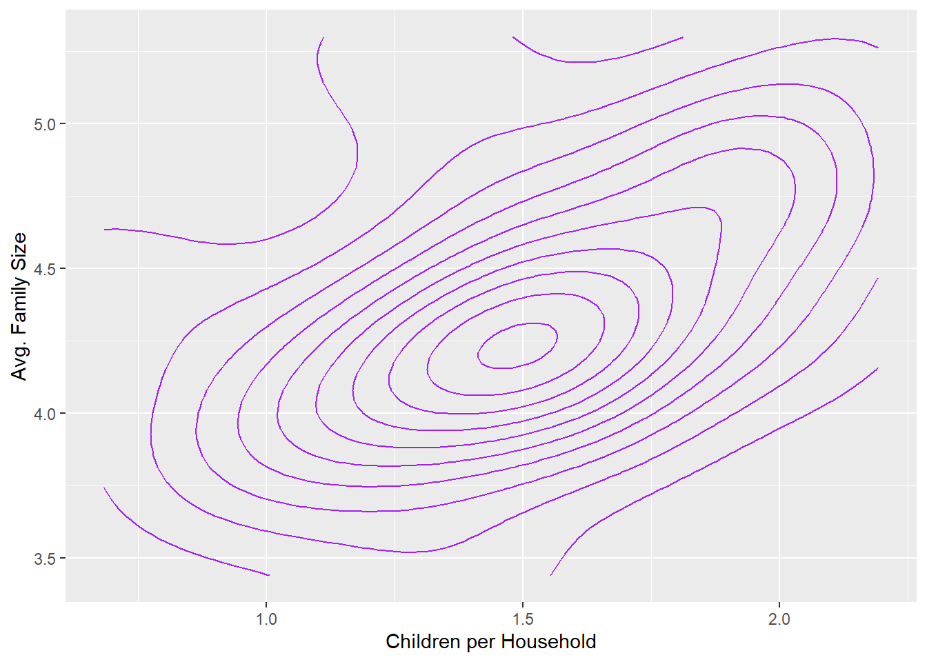
One nice aspect of a density plot is that it can make the correlation (or lack thereof) between two variables clearer. As we see here, the orientation of the gradient is diagonal, an observation that can sometimes be difficult to identify when distracted by outliers.
We can do the same for our second bivariate comparison as well.
child_by_imm+geom_density_2d(color = 'purple') +
  labs(x='Proportion of Immigrant Households',
       y='Children per Household')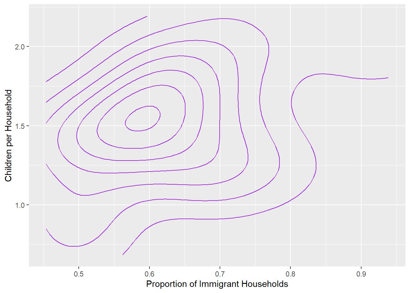
Again, the gradient is on a diagonal, though we can see the curve on the far right accommodating the outliers with extremely high proportions of immigrant households.
7.9 Summary
By aggregating records and merging the products, we created a data frame with a series of custom-designed quantitative measures describing a given unit of analysis, in this case the wards of Boston in 1880. While this might seem a somewhat obvious statement, it is actually the first time in this book that it is true! Previously, we have worked with data at the record level dominated by categorical variables and the occasional quantitative descriptor, be it temperature or precipitation during bike collisions or the price of apartments posted on Craigslist. Here instead we took census records and created measures to describe the population of each of Boston’s wards. The measures were of our design and reflected things that we wanted to know-—and therefore that we could easily interpret and describe. This is an important step in the ability to work with and communicate the content of any set of records.
In the process, we have developed the following skills, all of which are applicable to any aggregation effort, be it from records to individuals, individuals to households and neighborhoods, or otherwise:
- Aggregate records to higher units of analysis by using the
aggregate()command in base R, including:- Incorporating logical statements,
- Aggregating multiple variables with the same function,
- Aggregating on multiple key variables at once;
- Aggregate records to higher units of analysis by using the
group_by()andsummarise()commands intidyverse, including:- Incorporating logical statements,
- Aggregating multiple variables using a variety of functions and equations,
- Aggregating on multiple key variables at once;
- Merge separate data frames on shared key variables using the
merge()function in base R; - Merge separate data frames on shared key variables using the family of
joinfunctions intidyverse; - Query and aggregate records from a data frame (or database) with SQL language, through the
sqldfpackage; - Create custom functions that could then be called in aggregations or other commands requiring statistical functions;
- Visualize bivariate relationships between numerical variables using
geom_point()andgeom_density2d().
7.10 Exercises
7.10.1 Problem Set
- Suppose you are working with the data set used for the worked example in this chapter. Write code for creating each of the following aggregations in base R,
tidyverse, and SQL. Briefly explain the logic for each.- Proportion of immigrants in ward.
- Female-headed household.
- Proportion of female-headed households in a ward.
- You have two data frames of census blocks:
blocksandcblocks.The first has the unique identifier for each block asBlk_ID. The second has the same information inFIPS, which is a common label in census data.- Write code to merge these data frames. Briefly explain your reasoning.
- The first has blocks for the whole state, the other is just greater Boston. How does your merge generate each of the following outcomes:
- All census blocks.
- Only the census blocks in greater Boston.
- You have two data frames with
Blk_ID, each with 100 rows. You merge them and get 178 rows. How might this have happened? How would you attempt to fix it?
7.10.2 Exploratory Data Assignment
Working with a data set of your choice:
- Create new measures based on aggregations of your data. If you are working with the same data set across chapters, you can use this as an opportunity to begin calculating the latent constructs that you proposed in the Exploratory Data Assignment in Chapter 6.
- Be sure to describe why each measure is interesting and how the specific calculations you are using capture it. In addition, if these are intended as manifest variables of one or more latent constructs, describe how they are reflective of this underlying construct.
- Describe the content of these new variables statistically and graphically using tools we have learned throughout the book. Be sure to include at least one dot plot that shows the relationships between two variables at the aggregate level.