3 Telling a Data Story: Examining Individual Records
In the early 2000’s, New York City’s 311 system received a call from a constituent about a “strange maple syrup smell.” Needless to say, this did not fit a standard case type, like graffiti, streetlight outage, or pothole. And then the City received another such call. And another. And then dozens more. While complaining about a smell reminiscent of pancakes and waffles might seem a little silly, its unfamiliarity combined with a post-9/11 mentality convinced some that it was a harbinger of a chemical attack on the city. For 4 years, the smell and the resultant calls came and went, appearing in one neighborhood on one day, in another neighborhood a few weeks later, and so on.
In January 2009, when the smell appeared again in northern Manhattan, New York City’s government took decisive action. It realized that each of these 311 reports was a data story communicating precise information about when and where the odor was occurring. As a composite, these many complaints might allow them to pinpoint what the smell was and where it was coming from. As illustrated in Figure 3.1, they mapped out the reports, combined them with detailed weather data, and voila! It seemed apparent that the smell was coming from a set of factories in northern New Jersey, which, as it happened, fabricated (among other things) a chemical extract from fenugreek seeds. And what, might you ask, did that tell them? Fenugreek seeds are the primary source of flavoring for synthetic maple syrup. Case closed.
This tale encapsulates so much about the practice of urban informatics . A team of analysts leveraged a naturally occurring data set—one that was intended to support administrative processes, not necessarily research ventures—in creative ways to answer a real-world problem that was unnerving (if not quite threatening) the neighborhoods of New York City. They became modern age detectives by looking closely at the data records generated by the 311 system and recognizing the data story they could tell. Each record is a discrete piece of information, rife with details and clues about an event or condition occurring at a place and time. Understanding the information locked within this content is the secret not only to interpreting individual records, but also knowing what can be learned from the thousands or even millions that populate a full data set.
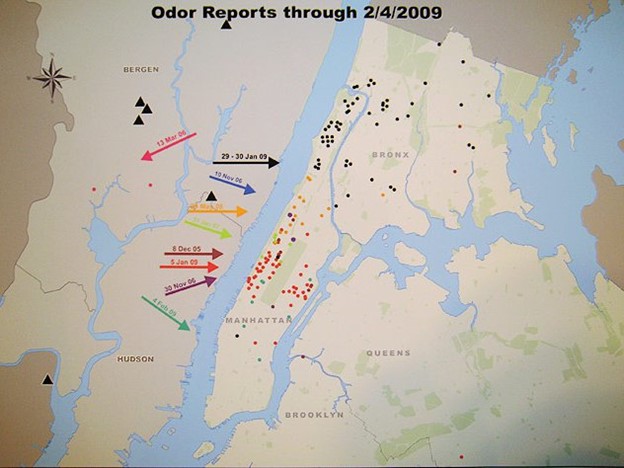
Figure 3.1: After years of investigation, in 2009 New York City officials combined 311 reports of a mysterious maple syrup smell (dots) with historical data on wind direction and speed (arrows) to determine that the odor was coming from factories that process artificial flavoring for maple syrup. (Credit: Gothamist)
In this chapter, we are going to learn the basic skills needed to “tell a data story” from individual records. It might seem a little simplistic to spend an entire chapter looking at individual records—the whole point of this book is to analyze big, complex data sets, right? But becoming acquainted with the content of individual records is a crucial first step to being able to make sense of the opportunities (and challenges) of the full data set. Rest assured that we will build toward that by the next chapter.
3.1 Worked Example and Learning Objectives
Boston has a 311 system as well. Though it has never been used to solve a Maple Syrup Mystery, it has all sorts of other content that lends itself to investigation. We will use it to learn how to tell data stories, including the following skills:
- Use RMarkdown as a special scripting file for sharing both our code and results;
- Access and import datasets into R;
- Subset data to scrutinize specific records in both base R and
tidyverse; - Leverage other tools for systematically exposing records, including sorting;
- Think critically about the content of a data record and its interpretation.
3.1.1 Getting Started - A Reminder
This and all worked examples following it will assume that you have booted up RStudio and opened the desired project. You may want to have a separate project for each chapter or unit, or just have a single project running through the book—whatever works best for your style of organization. If you need to refresh on how to create a project, you are always welcome to flip back to Chapter 2. This will be the last time this reminder appears in the book.
3.2 Introducing R Markdown
In Chapter 2, we learned about scripts as a way to write and save code. Scripts allow us to write out multistep processes and send them to the console for execution at our desired pace. They also make it possible to easily share our manipulations and analyses with our colleagues (and the general public, if so desired). But imagine if you could share not only your code but also the results. A reader could then rerun the code and know if the results were the same or read the results and know precisely how you got there. There is a tool that does precisely this.
R Markdown is a special type of script in R that embeds executable chunks of code, each followed by the results they generate, in a single document. This process is referred to as “knitting,” as it interweaves the code and its results together. As you might imagine, it is powered by additional packages, most prominently knitr. It can export the resulting document in HTML and pdf formats, among others. This book, in fact, is written in an extension of R Markdown called Bookdown.
Getting started with Markdown is simple. Just as we did for a new script, click in the upper left-hand corner on the ‘New’ button
this time selecting “R Markdown…”. (You will probably be prompted to install a bunch of packages. Just click Yes.) You will see an interface like this:
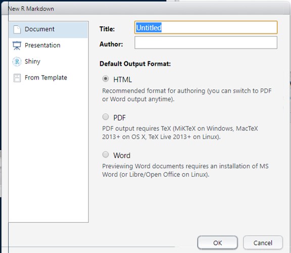
Name your document (give it an author if you like). I tend to keep HTML as the standard output; this is ideal especially if you want to post on the web at any point. The left-hand options give a sense of the other type of formats that Markdown can support, but we will stick with Document.
You should now have a new script, but one that looks a little different:
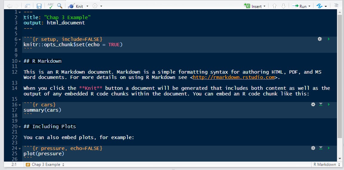
This R Markdown, or .Rmd, script comes prepopulated with some text. A few things to note.
There is a title and output as you specified when you created the file. These will inform how the final document is knitted (e.g., the title will be placed at the top).
The document consists of plain text (black background in the figure) and code (on a lighter gray-blue background in the figure). Three backwards accents or tick marks (
```) followed by brackets with the letter and then additional text ({r}) indicates the start of a chunk using R syntax and the title for the chunk, and the next three backwards accents (```) indicate the end of a chunk. R will execute each chunk as a single block of code and report all results in order underneath it. The plain text will appear as text in between the chunks in the final document.Third, the default summary text references clicking the Knit button just above the script as the step for generating a document. This button will offer the standard format options for knitting.

3.3 Access and Import Data
Let’s get started for real! First, we need to visit the City of Boston’s Open Data Portal and download 311 data. When you go to Analyze Boston, you will be presented with a search box:

Enter “311” into the box. Your first option should be “311 Service Requests.” This will lead us to a collection of data files included under 311 Service Requests—you can think of the latter as a file folder holding all of these files. Note that the City of Boston has smartly divided the data into annual files. If they were combined they would be rather large. They also have published a documentation file in a .pdf, called the CRM Value Codex (CRM, or Constituent Relationship Management, system is another name for 311). We will not need that here, but if you want to dig into the data further, I suggest you read it.
For this exercise, we will download 311 Service Requests – 2020. The default title of the data set is a bit messy. If you choose to rename it (which I have done), you will want to do so by right-clicking on the file (or clicking with two fingers on a Mac) and selecting rename. DO NOT ATTEMPT TO OPEN IN EXCEL AND RESAVE AS THIS CAN ALTER THE CONTENT OF THE DATA SET. Save the data set in the directory of the project with which you are working in RStudio.
To import the data, return to your RStudio. There is a point-and-click way to import data, but we are going to do so using code as this is good practice. Remember that code allows us to specify exactly what we want R to do and allows us to communicate to others what we did. Importing data occurs through the read.csv command, because the data are in a .csv or comma separated values format, which is the most accessible format for transferring data across programs:
read.csv('Boston 311 2020.csv' , na.strings=c(''))
(I have had to add the additional argument na.strings owing to a quirk in the Boston data file. This ensures that blank values will be converted to NA, which is the standard in R.) If your file is in the same folder as your project, then simply entering its name will be sufficient. If it is in another folder, you will need to enter the folder directory as well:
read.csv('C:/Users/dobrien/OneDrive - Northeastern University/Documents/Textbook/Unit 1 - Information/Chapter 3 - Telling a Data Story/Example/Boston 311 2020.csv', na.strings=c(''))
You may be surprised here to see the use of / rather than \ in the file directory. This is because R syntax uses \ for other purposes, so if you copy-and-paste your directory you will need to flip the slashes.
We can enter this line of code from your Rmd using ctrl+Enter or by pressing the green arrow at the top-right of the chunk (the gear on the left is for options, and the down arrow is for running all chunks).

In either case, you should see the first 34 of 251,374 rows (or observations). This is rather large so I have not printed it here. But notice that nothing appeared in our Environment. This is because we did not store the imported data in an object. Let’s try again:
bos_311<-read.csv('C:/Users/dobrien/OneDrive - Northeastern University/Documents/Textbook/Unit 1 - Information/Chapter 3 - Telling a Data Story/Example/Boston 311 2020.csv', na.strings=c(''))
This time, nothing was outputted in the Markdown, but a data frame with 251,374 observations and 29 variables with the name bos_311 appeared in the Environment. Success! (You are welcome to name the data frame anything you want when you import.) Importantly, if we are using read.csv(), R assumes we will store the imported content as a data frame. Also, note that if read.csv() is instructed to store the imported data in a new object, nothing is printed out, which is why we do not see any output.
read.csv() is the most commonly used import command in R and the one we will use almost exclusively in this book. There are other versions of the read command for other data formats (e.g., read.table(), read.fortran(), read.delim()). It may be disappointing to learn, however, that files from Excel (.xlsx) and other proprietary programs (including SAS, Stata, and SPSS) are not easily imported into R because of their highly specific encoding. As such, if you want to transfer data from these programs into R, you are best off saving them as .csv and importing them that way.
3.4 Getting Acquainted with a Data Frame’s Structure
When we first import a data set, we may want to get a better sense of its structure to guide our explorations. Some tools for this include
dim(bos_311)## [1] 251374 29This tells us what we already know from the Environment, the data set contains 251,374 observations and 29 columns. We can also break this up with the nrow() and ncol() commands, which produce each of those pieces of information separately.
We may also want a preliminary sense of the types of information contained in the data set. The names() function gives us exactly that.
names(bos_311)## [1] "case_enquiry_id"
## [2] "open_dt"
## [3] "target_dt"
## [4] "closed_dt"
## [5] "ontime"
## [6] "case_status"
## [7] "closure_reason"
## [8] "case_title"
## [9] "subject"
## [10] "reason"
## [11] "type"
## [12] "queue"
## [13] "department"
## [14] "submittedphoto"
## [15] "closedphoto"
## [16] "location"
## [17] "fire_district"
## [18] "pwd_district"
## [19] "city_council_district"
## [20] "police_district"
## [21] "neighborhood"
## [22] "neighborhood_services_district"
## [23] "ward"
## [24] "precinct"
## [25] "location_street_name"
## [26] "location_zipcode"
## [27] "latitude"
## [28] "longitude"
## [29] "source"From here we can see there are multiple variables about timing, including when a case was opened (open_dt) and closed (closed_dt), whether it was completed on time (ontime), the type of issue reported (type), where the issue occurred (location) and its neighborhood (neighborhood), among other things.
We can also find out more about each of these variables using the class() command. This requires isolating a single variable with what is called dollar-sign notation, taking the form df$column (we will do much more of this later in the chapter).
class(bos_311$neighborhood)## [1] "character"tells us that the neighborhood variable is, unsurprisingly a character variable and
class(bos_311$case_enquiry_id)## [1] "numeric"tells us that case_enquiry_id is a numeric variable, reflecting its role as a serial number to identify unique reports.
If we want to see all cases from the top of the data frame, we can use
head(bos_311)## case_enquiry_id open_dt target_dt
## 1 101003157986 2020-01-13 08:58:29 2020-04-12 08:58:29
## 2 101003158274 2020-01-13 11:53:00 2020-02-12 11:53:46
## 3 101003152474 2020-01-06 14:15:00 2020-01-07 14:15:39
## 4 101003154625 2020-01-08 15:39:00 2020-02-07 15:39:25
## 5 101003160351 2020-01-15 11:09:00 2020-01-16 11:09:05
## 6 101003160360 2020-01-15 11:10:00 2020-05-14 11:10:27
## closed_dt ontime case_status closure_reason
## 1 <NA> OVERDUE Open
## 2 <NA> OVERDUE Open
## 3 <NA> OVERDUE Open
## 4 <NA> OVERDUE Open
## 5 <NA> OVERDUE Open
## 6 <NA> OVERDUE Open
## case_title subject
## 1 Rental Unit Delivery Conditions Inspectional Services
## 2 Heat - Excessive Insufficient Inspectional Services
## 3 Unsafe/Dangerous Conditions Inspectional Services
## 4 Rodent Activity Inspectional Services
## 5 Pick up Dead Animal Public Works Department
## 6 Unsatisfactory Living Conditions Inspectional Services
## reason type
## 1 Housing Rental Unit Delivery Conditions
## 2 Housing Heat - Excessive Insufficient
## 3 Building Unsafe Dangerous Conditions
## 4 Environmental Services Rodent Activity
## 5 Street Cleaning Pick up Dead Animal
## 6 Housing Unsatisfactory Living Conditions
## queue department
## 1 ISD_Housing (INTERNAL) ISD
## 2 ISD_Housing (INTERNAL) ISD
## 3 ISD_Building (INTERNAL) ISD
## 4 ISD_Environmental Services (INTERNAL) ISD
## 5 INFO_Mass DOT INFO
## 6 ISD_Housing (INTERNAL) ISD
## submittedphoto closedphoto
## 1 <NA> <NA>
## 2 <NA> <NA>
## 3 <NA> <NA>
## 4 <NA> <NA>
## 5 <NA> <NA>
## 6 <NA> <NA>
## location
## 1 40 Stanwood St Dorchester MA 02121
## 2 9 Wayne St Dorchester MA 02121
## 3 21-23 Monument St Charlestown MA 02129
## 4 98 Everett St East Boston MA 02128
## 5 INTERSECTION of Frontage Rd & Interstate 93 N Roxbury MA
## 6 6 Rosedale St Dorchester MA 02124
## fire_district pwd_district city_council_district
## 1 7 03 4
## 2 9 10B 7
## 3 3 1A 1
## 4 1 09 1
## 5 4 1C 2
## 6 8 07 4
## police_district neighborhood
## 1 B2 Roxbury
## 2 B2 Roxbury
## 3 A15 Charlestown
## 4 A7 East Boston
## 5 C6 South Boston / South Boston Waterfront
## 6 B3 Dorchester
## neighborhood_services_district ward precinct
## 1 13 Ward 14 1401
## 2 13 Ward 12 1207
## 3 2 Ward 2 0204
## 4 1 Ward 1 0102
## 5 0 0 0801
## 6 9 Ward 17 1703
## location_street_name location_zipcode
## 1 40 Stanwood St 2121
## 2 9 Wayne St 2121
## 3 21-23 Monument St 2129
## 4 98 Everett St 2128
## 5 INTERSECTION Frontage Rd & Interstate 93 N NA
## 6 6 Rosedale St 2124
## latitude longitude source
## 1 42.3093 -71.0801 Constituent Call
## 2 42.3074 -71.0853 Constituent Call
## 3 42.3778 -71.0598 Constituent Call
## 4 42.3674 -71.0341 Constituent Call
## 5 42.3594 -71.0587 Citizens Connect App
## 6 42.2926 -71.0722 Constituent Callwhich shows the first 6 cases (though that can be modified; try, for example, head(bos_311,n=10)). The tail() command does the same for the end of the data set.
The str() command combines nearly all of these tools, reporting the number of rows and columns and a list of all variable names, their class, and the first few values for each. (Try it on your own. I’ve omitted it because it gets a little lengthy.)
Last, you may want to browse through the observations a little as though it were an Excel spreadsheet. You can do this with View(), as we did in the previous chapter.
3.5 Subsetting Data Objects
3.5.1 Subsetting Data: How and Why?
Recall that R is an object-oriented programming language , meaning functions are applied to data objects that can take a variety of forms (see Chapter 2 for a refresher). In practice, this means that all of R’s many functions are intended to manipulate and examine data objects to reveal or expose content in flexible ways. The most basic way to do this is to isolate and observe a subset of an object. This can be done for any data object. For now, we are going to learn how to do so in brief for vectors, and then in more depth for data frames. Importantly, R offers various tools that allow us to create subsets that reflect exactly the observations (and variables) we want to look at more closely.
Why is it useful to subset our data? The most basic answer is that we want to be able to scrutinize content more directly. We might want to make sense of the information contained in a single row or group of rows. We might want to check for anomalies that communicate the extremes of a data set or even errors that might be in it. We might want to use a closer look at multiple records to better understand the broader opportunities and challenges presented by the full data set. Those are our goals in this chapter, but they also lay the groundwork for ways that subsets will be useful in future chapters, often delimiting and targeting our analyses and visualizations to provide the specific insights that we are looking for.
3.5.2 Subsetting in Base R: Vectors
In base R, subsets are indicated by placing brackets after an object’s name, with the brackets containing criteria denoting the desired cases. The simplest example is with vectors. To illustrate, let us return to a vector constructed in Chapter 2:
bos_event_types<-c('311','Permits','Major Crimes')
bos_event_types[1]
## [1] "311"The bracket [1] instructed R to print the first element in the vector. Try again with [2] or [3]. What do you think will happen?
3.5.3 Subsetting in Base R: Data Frames
3.5.3.1 Subsetting by Values
The logic for subsetting data frames is similar to that for vectors, except that data frames have two dimensions on which we can subset: rows (observations) and columns (variables). Thus, the brackets need to specify what we want from each, with a comma in between. That is, we want [row,column], for instance,
bos_311[5,1]## [1] 101003160351This command gives us the case_enquiry_id (a serial number identifying the report; the first column) for the fifth observation (View() or click on the data frame in the Environment to check, if you like). We might also see its open_dt (the date and time the report was received; column #2).
bos_311[5,2]## [1] "2020-01-15 11:09:00"which was January 15th, 2020 at 11:09 am.
What if we want to see the entirety of the case to tell its story? We need to enter a row without columns specified. The following code will generate the desired case and its values for all columns
bos_311[5,]## case_enquiry_id open_dt target_dt
## 5 101003160351 2020-01-15 11:09:00 2020-01-16 11:09:05
## closed_dt ontime case_status closure_reason
## 5 <NA> OVERDUE Open
## case_title subject reason
## 5 Pick up Dead Animal Public Works Department Street Cleaning
## type queue department submittedphoto
## 5 Pick up Dead Animal INFO_Mass DOT INFO <NA>
## closedphoto
## 5 <NA>
## location
## 5 INTERSECTION of Frontage Rd & Interstate 93 N Roxbury MA
## fire_district pwd_district city_council_district
## 5 4 1C 2
## police_district neighborhood
## 5 C6 South Boston / South Boston Waterfront
## neighborhood_services_district ward precinct
## 5 0 0 0801
## location_street_name location_zipcode
## 5 INTERSECTION Frontage Rd & Interstate 93 N NA
## latitude longitude source
## 5 42.3594 -71.0587 Citizens Connect AppNow we are getting somewhere, and possibly somewhere interesting. We see that the case was reported on January 15th, 2020 (open_dt), and the City indicated that it should be closed by the next day (target_dt). However, it was never closed (closed_dt is empty) and it is flagged as being OVERDUE (ontime) and Open (case_status).
Rmd limits to the first six variables. If we wanted to learn even more, we could do View(bos_311[5,]) and find out that it was a request to Pick up Dead Animal (type) at the INTERSECTION of Frontage R & Interstate 93 N (location) in South Boston / South Boston Waterfront (neighborhood). Note how these pieces of information fit together to tell a story. What do you think happened here?
You will notice that R needed us to put a comma after the 5 to know that we wanted row 5. If you entered bos_311[5] it would have assumed that you wanted column 5. That is, as a default, R is designed to assume that analysts are more likely to want to see all cases on a subset of variables than all variables on a subset of cases. bos_311[,5] would accomplish the same outcome.
Selecting a single value or a single row or column is only so useful. There are multiple ways for us to expand this while still working exclusively with numbers.
Colons allow us to indicate a series of consecutive values. For instance,
bos_311[1:4,]would generate all variables for the first four cases, andbos_311[4:10,]would generate the same for cases 4-10.c(), or the combine command, can put together non-consecutive values. For example,bos_311[c(1,2,4:6),]would return all variables for cases 1, 2, 4, 5, and 6. Meanwhile,bos_311[c(1,2,4:6)]would generate variables 1, 2, 4, 5, and 6 for all cases.
If you like, this is a good time to play around with some options and to check them against the data set to confirm that you are comfortable with subsetting by row and column values.
3.5.3.2 Subsetting Columns
There are two other ways to subset columns that can feel more accessible. The first is by name.
head(bos_311['neighborhood'])## neighborhood
## 1 Roxbury
## 2 Roxbury
## 3 Charlestown
## 4 East Boston
## 5 South Boston / South Boston Waterfront
## 6 DorchesterSee how this lists the neighborhood where each event reported to 311 occurred. We can also combine multiple variables using this notation.
head(bos_311[c('neighborhood','type')])## neighborhood
## 1 Roxbury
## 2 Roxbury
## 3 Charlestown
## 4 East Boston
## 5 South Boston / South Boston Waterfront
## 6 Dorchester
## type
## 1 Rental Unit Delivery Conditions
## 2 Heat - Excessive Insufficient
## 3 Unsafe Dangerous Conditions
## 4 Rodent Activity
## 5 Pick up Dead Animal
## 6 Unsatisfactory Living Conditionsgenerates the list of neighborhoods and the case types for all observations. This notation is compatible with subsets of observations as well:
bos_311[5,c('neighborhood','type')]## neighborhood type
## 5 South Boston / South Boston Waterfront Pick up Dead Animalgenerates these two pieces of information for observation #5.
The second way is with dollar-sign notation. This notation takes the form df$column and can only isolate a single variable:
head(bos_311$neighborhood)## [1] "Roxbury"
## [2] "Roxbury"
## [3] "Charlestown"
## [4] "East Boston"
## [5] "South Boston / South Boston Waterfront"
## [6] "Dorchester"generates the same information as bos_311 (though the first stays within Rmd, the latter generates more extensive results in the Console).
Though it is not possible to select multiple variables this way, it is possible to simultaneously subset by rows and columns. Remember that each column in a data frame is actually a vector. So, when we subset “rows” with dollar-sign notation, we are actually subsetting a vector. This means we do not need the comma.
bos_311$neighborhood[5]## [1] "South Boston / South Boston Waterfront"This tells us again that this case occurred in the South Boston / South Boston Waterfront neighborhood.
3.5.3.3 Subsetting with Logical Statements
The last way to subset is by using logical statements based on the content of the data. This can be very powerful when we want to target our analyses based on specific criteria. For example, what if we want to see all cases that were still open when the data set was posted? (Limiting to the first six variables for brevity’s sake.)
head(bos_311[bos_311$case_status=='Open',1:6])## case_enquiry_id open_dt target_dt
## 1 101003157986 2020-01-13 08:58:29 2020-04-12 08:58:29
## 2 101003158274 2020-01-13 11:53:00 2020-02-12 11:53:46
## 3 101003152474 2020-01-06 14:15:00 2020-01-07 14:15:39
## 4 101003154625 2020-01-08 15:39:00 2020-02-07 15:39:25
## 5 101003160351 2020-01-15 11:09:00 2020-01-16 11:09:05
## 6 101003160360 2020-01-15 11:10:00 2020-05-14 11:10:27
## closed_dt ontime case_status
## 1 <NA> OVERDUE Open
## 2 <NA> OVERDUE Open
## 3 <NA> OVERDUE Open
## 4 <NA> OVERDUE Open
## 5 <NA> OVERDUE Open
## 6 <NA> OVERDUE OpenYou should see in your Rmd the first 6 of 34,836 rows and 6 of 29 columns, as well as a 7th column at the front. This is the row name, which is most often an index of the original order of cases. Also note that case_status indeed is equal to Open for all cases.
How did this work? First, we needed to indicate the variable that would be the basis for the criterion, bos_311$case_status. We then needed to define the criterion as being equal to Open, which is in single quotations because it is text. In R, “equal to” in a criterion is not represented with a single equals sign but with two in a row (==). This is because a single equals sign sets one thing equal to another. We want to actually evaluate whether the two things are equal. In a sense, you might think of it as asking the computer, “Is it true (i.e., equal to reality) that these two things are equal?” Then, of course, we need a “,” at the end to indicate that we want all rows equal to this criterion.
From a technical perspective, here is what is happening. R is evaluating whether case_status is equal to ‘Open’ for every case in the data set. It then assigns each a TRUE or FALSE value and creates a list of observation numbers for which TRUE is the case. It then uses this list to create the subset. Thus, R figured out that what we wanted was bos_311[c(1:7, 19, 22, 41, …),]. You, of course, would not have known to ask for this unless you had evaluated every case to know whether it was still Open or not, but R did this for you.
An advantage of logical statements is the ability to create more than one criterion. One striking thing here is that case 22 appears to be ONTIME although still Open since January 1st, 2020. How common is it for these two things to be true? Let’s find out by using the & operator to indicate multiple criteria.
head(bos_311[bos_311$case_status=='Open' &
               bos_311$ontime=='ONTIME',1:6])
## case_enquiry_id open_dt target_dt
## 22 101003148513 2020-01-01 15:02:00 <NA>
## 62 101003148723 2020-01-02 07:03:00 <NA>
## 72 101003148792 2020-01-02 08:09:00 <NA>
## 83 101003148854 2020-01-02 08:55:00 <NA>
## 124 101003149184 2020-01-02 11:53:00 2021-12-22 11:53:26
## 152 101003149460 2020-01-02 14:45:00 2021-12-22 14:45:03
## closed_dt ontime case_status
## 22 <NA> ONTIME Open
## 62 <NA> ONTIME Open
## 72 <NA> ONTIME Open
## 83 <NA> ONTIME Open
## 124 <NA> ONTIME Open
## 152 <NA> ONTIME OpenThere are 13,512 such cases. Looking at the top of the data set, it appears that many of these had no target_dt to be benchmarked against. Hard to be OVERDUE if you had no due date. But there are some others for which the targets are very far away, in December 2021, meaning they had not been due yet at the time of the export of the data (though if you are doing this exercise after December 2021, the data might look a little different).
Is it possible this is true for certain case types? We could create a subset to examine this, too. Maybe we can learn more about this by limiting to those cases without target dates. This will use a new function called is.na(), which identifies all cases with the value of NA for a given variable:
head(bos_311[bos_311$case_status=='Open' &
               bos_311$ontime=='ONTIME' &
               is.na(bos_311$target_dt),1:6])
## case_enquiry_id open_dt target_dt closed_dt
## 22 101003148513 2020-01-01 15:02:00 <NA> <NA>
## 62 101003148723 2020-01-02 07:03:00 <NA> <NA>
## 72 101003148792 2020-01-02 08:09:00 <NA> <NA>
## 83 101003148854 2020-01-02 08:55:00 <NA> <NA>
## 177 101003149654 2020-01-02 19:04:00 <NA> <NA>
## 214 101003150009 2020-01-03 09:29:00 <NA> <NA>
## ontime case_status
## 22 ONTIME Open
## 62 ONTIME Open
## 72 ONTIME Open
## 83 ONTIME Open
## 177 ONTIME Open
## 214 ONTIME OpenWhen we do this, we find that quite a few of those without target dates are about animals or are general informational requests, which might mean that it is hard to set a target when you cannot be sure that said animal will still be there or for something informational.
head(bos_311[is.na(bos_311$target_dt),c('target_dt','case_status',
                                        'ontime','type')])
## target_dt case_status ontime type
## 22 <NA> Open ONTIME Animal Generic Request
## 26 <NA> Closed ONTIME Needle Pickup
## 27 <NA> Closed ONTIME Needle Pickup
## 29 <NA> Closed ONTIME Needle Pickup
## 30 <NA> Closed ONTIME Needle Pickup
## 31 <NA> Closed ONTIME Needle PickupNote that only one of these at the top is animal related, and most are needle pickups. Happily, those were all Closed.
3.5.3.4 Extra Tools for Subsetting
This exercise has shown a good bit about how to subset, but there are two final skills we want to leave with. The first is the ! operator, which means “not equal” in R. In the spirit of the double equals sign, though, it needs to be applied to something, in this case an equals sign. For instance,
head(bos_311[bos_311$case_status!='Open',1:6])## case_enquiry_id open_dt target_dt
## 8 101003172959 2020-01-19 06:44:00 2020-01-28 08:30:00
## 9 101003148263 2020-01-01 03:27:00 2020-01-02 03:27:09
## 10 101003148269 2020-01-01 06:19:00 2020-01-03 08:30:00
## 11 101003148271 2020-01-01 07:02:00 2020-01-03 08:30:00
## 12 101003148342 2020-01-01 10:50:00 2020-01-31 10:50:14
## 13 101003148276 2020-01-01 07:56:41 2020-01-03 08:30:00
## closed_dt ontime case_status
## 8 2020-02-03 14:04:40 OVERDUE Closed
## 9 2020-01-06 08:03:45 OVERDUE Closed
## 10 2020-01-02 06:10:56 ONTIME Closed
## 11 2020-01-01 07:07:17 ONTIME Closed
## 12 2020-01-03 10:57:38 ONTIME Closed
## 13 2020-01-02 05:08:04 ONTIME Closedunsurprisingly generates a subset of all cases that are Closed, meaning not equal to Open.
Or
head(bos_311[!is.na(bos_311$target_dt),1:6])## case_enquiry_id open_dt target_dt
## 1 101003157986 2020-01-13 08:58:29 2020-04-12 08:58:29
## 2 101003158274 2020-01-13 11:53:00 2020-02-12 11:53:46
## 3 101003152474 2020-01-06 14:15:00 2020-01-07 14:15:39
## 4 101003154625 2020-01-08 15:39:00 2020-02-07 15:39:25
## 5 101003160351 2020-01-15 11:09:00 2020-01-16 11:09:05
## 6 101003160360 2020-01-15 11:10:00 2020-05-14 11:10:27
## closed_dt ontime case_status
## 1 <NA> OVERDUE Open
## 2 <NA> OVERDUE Open
## 3 <NA> OVERDUE Open
## 4 <NA> OVERDUE Open
## 5 <NA> OVERDUE Open
## 6 <NA> OVERDUE Opengenerates all cases for which target_dt has a value, some of which have closed dates, some of which do not.
Second, sometimes we do not want the combination of criteria but their intersection. This requires an ‘or’ statement, which uses the | symbol (over on the far right under Backspace on most English keyboards). Suppose we want to know about all cases that are either OVERDUE or have never been closed, because the latter can slip by unnoticed if there was no target date.
head(bos_311[is.na(bos_311$closed_dt) |
               bos_311$ontime=='OVERDUE',1:6])
## case_enquiry_id open_dt target_dt
## 1 101003157986 2020-01-13 08:58:29 2020-04-12 08:58:29
## 2 101003158274 2020-01-13 11:53:00 2020-02-12 11:53:46
## 3 101003152474 2020-01-06 14:15:00 2020-01-07 14:15:39
## 4 101003154625 2020-01-08 15:39:00 2020-02-07 15:39:25
## 5 101003160351 2020-01-15 11:09:00 2020-01-16 11:09:05
## 6 101003160360 2020-01-15 11:10:00 2020-05-14 11:10:27
## closed_dt ontime case_status
## 1 <NA> OVERDUE Open
## 2 <NA> OVERDUE Open
## 3 <NA> OVERDUE Open
## 4 <NA> OVERDUE Open
## 5 <NA> OVERDUE Open
## 6 <NA> OVERDUE OpenThese are just some initial examples. We can of course get into more complicated criteria, with any number of &s and |s, though it takes some critical thinking to determine exactly what order you want them to be in and whether you need parentheses to set some off from others, or whether a ! should be in there somewhere.
3.5.3.5 Summary
Because we have gained a variety of skills for subsetting in R through a worked example, it is useful to pause and reflect on what we learned.
- We can subset vectors and data frames.
- Subsetting data frames can occur using values in brackets with
[row,column]. - The values in the brackets can be expanded using a colon for consecutive values, and
c()for non-consecutive values. - We can isolate single variables with
df$columnand multiple variables with quotations within brackets. - We can use logical statements to create subsets according to criteria, including:
==for equal to!=for not equal tois.na()for blank cases&to combine criteria and|to identify cases in which either of two criteria are true (an or statement).- All of these can be combined flexibly to define the exact subset that you want.
3.5.4 Subsetting in tidyverse
As discussed in Chapter 2, many of the skills we will learn in Base R have parallels in tidyverse, a set of packages designed to make coding in R cleaner (or more “tidy,” as the name implies). These parallels are often simpler to work with. We will see this for the first time by learning how to subset in tidyverse. If you have not already installed tidyverse and its underlying packages, you can do so with the command install.packages(‘tidyverse’). To get started with this part of the worked example, you will then need to
require(tidyverse)First, it is worth noting that tidyverse commands convert dataframes into “tibbles.” Tibbles are essentially data frames with a few small technical tweaks that we do not need to delve into here, but you can learn more about them in the tidyverse documentation at www.tidyverse.org.
Turning to subsetting in tidyverse, there are two main functions that we can use: filter() and select(). The first subsets rows, the latter subsets columns. We will also need to learn a third skill called “piping” to combine them. We can illustrate all three with code from our worked example. (Note: for brevity, I will not have the subsets in this section print out. You are welcome, though, to check that the Base R and tidyverse versions agree.)
3.5.4.1 filter()
When we wanted to see all Open cases, we entered
head(bos_311[bos_311$case_status=='Open',])We can do the same with the filter() command, which takes the form filter(df, criteria) as
head(filter(bos_311, case_status=='Open'))You will notice that we no longer have brackets after the name of the data frame. Instead, we are telling R the name of the data frame in the first argument, and then giving it the criteria in the second argument. Because filter specifically handles rows, we also no longer need the comma at the end. Last, because the first argument already indicates the data frame of interest, we can refer directly to variables therein without dollar-sign notation.
The same process would apply to one of our more complex criteria:
head(bos_311[is.na(bos_311$closed_dt) | bos_311$ontime=='OVERDUE',])becomes
head(filter(bos_311, is.na(closed_dt) | ontime=='OVERDUE'))But one other difference is that each & is replaced by a comma. You can think of it as entering a list of shared criteria.
bos_311[bos_311$case_status=='Open' & bos_311$ontime=='ONTIME',]becomes
filter(bos_311, case_status=='Open', ontime=='ONTIME')3.5.4.2 select()
The select() command subsets according to columns, and is structured in the same way as filter() with select(df, variable names). Thus
bos_311['neighborhood']and
bos_311$neighborhoodin Base R are equivalent to
select(bos_311,neighborhood)in tidyverse.
And
bos_311[c('neighborhood','type')]in Base R is equivalent to
select(bos_311,neighborhood, type)in tidyverse. Again, the first argument, which is the name of the data frame, removes the need for dollar-sign notation or quotation marks. R already knows that it is looking for variables within that data frame.
There are also multiple valuable helper functions that can be useful, especially in a data set with many variables that have similar structures (e.g., ends_with(dt) could be useful for isolating all variables that end with the suffix _dt, thereby referring to a date and time; starts_with() and contains() offer similar opportunities).
An additional trick is if you want to select all columns but exclude one or more, you can use a minus sign. For instance
View(select(CRM, -neighborhood, -type))selects all variables except for neighborhood and type.
3.5.4.3 Piping
Unfortunately, select() and filter() cannot be directly combined the way that brackets allow us to subset rows and columns at the same time. This can be solved, however, with a special capacity of tidyverse called “piping,” which “passes” the product of one command directly to another command. This allows the analyst to combine multiple manipulations in a series. Often it is possible to do something similar in Base R in a single line by nesting functions within each other, but it can get complicated and difficult to ascertain whether everything is just as we want it. Piping allows this process and its outcomes to be more easily examined.
Piping depends on the pipe symbol, %>%. We simply place it at the end of a line and the product of that code is passed to the next line. R does not conclude the steps until it reaches a line that does not end with a pipe. In theory, you can connect any number of lines with pipes, but it is typically best practice to keep them under 10; otherwise the complexity may merit breaking things up into pieces.
Let us demonstrate piping with select() and filter() for a few of the subsets we created above.
bos_311[bos_311$case_status=='Open' &
          bos_311$ontime=='ONTIME',
        c('target_dt','ontime','type')]
becomes
bos_311 %>%
  filter(case_status=='Open', ontime=='ONTIME') %>%
  select(target_dt,ontime,type)
The first line of a series of piped commands is often just the data frame of interest. When we say that pipes “pass” the product of the previous command, we mean the product of one command becomes the first argument of the next command. Thus, we do not need to restate the data frame for filter(). We skip straight to the criteria for rows that we want. After filter() is completed, the subset of rows is passed to select(), which narrows down to our three desired variables.
This is also an illustration of the importance of order. If we changed the order of filter() and select(), we get an error. Why? Feel free to think about it for a moment before reading on.
If we give select() first, we have already removed all variables except for target_dt, ontime, and type. As such, we can no longer filter() based on the content of case_status because no such variable exists.
This simple example demonstrates the elegance of piping, which we will use regularly when coding with tidyverse.
3.5.5 Combining Subsets with Other Tools
Immediately after importing our data, we learned a series of tools for exposing the structure of a data frame. We can utilize these effectively for any subset, as well, which could be informative. The most obvious might be for viewing a subset more closely
View(bos_311[bos_311$case_status=='Open' &
               bos_311$ontime=='ONTIME',
             c('target_dt','ontime','type')])
Now we can browse through all 13,512 rows in our subset rather than being limited to the first few.
Even simpler
nrow(bos_311[bos_311$case_status=='Open' &
               bos_311$ontime=='ONTIME',
             c('target_dt','ontime','type')])
## [1] 13512tells us that there are 13,512 rows in the subset without requiring us to generate the full subset.
To do the same thing in tidyverse, we add the new command to the end of the existing commands, though they will remain empty because we are passing the desired data frame directly to them:
bos_311 %>%
  filter(case_status=='Open', ontime=='ONTIME') %>%
  select(target_dt,ontime,type) %>%
  nrow()
## [1] 13512Try to do the same with View().
3.6 Sorting
A final skill we might want to leverage when exploring a new data set is sorting, which allows us to get a sense of the content of variables, especially their extreme values. Doing so in Base R is more complicated than you might expect, however. Let’s say we want to see the top of our data frame in order of the open dates for all cases, we need to enter
head(bos_311[order(bos_311$open_dt),1:6])## case_enquiry_id open_dt target_dt
## 220012 101003148236 2020-01-01 00:13:06 2020-01-03 08:30:00
## 45692 101003148237 2020-01-01 00:20:09 2020-01-03 08:30:00
## 9196 101003148238 2020-01-01 00:24:00 2020-01-03 08:30:00
## 15497 101003148239 2020-01-01 00:28:07 2020-03-09 08:30:00
## 220013 101003148240 2020-01-01 00:29:06 2020-01-03 08:30:00
## 754 101003148242 2020-01-01 00:31:00 2020-01-09 08:30:00
## closed_dt ontime case_status
## 220012 2020-01-02 03:12:46 ONTIME Closed
## 45692 2020-01-02 03:10:50 ONTIME Closed
## 9196 2020-01-01 01:20:40 ONTIME Closed
## 15497 <NA> OVERDUE Open
## 220013 2020-01-02 03:11:25 ONTIME Closed
## 754 <NA> OVERDUE OpenSubstantively we have learned that the 2020 data begin early in the morning on January 1st, 2020, which would seem a bit obvious, but is at least a good sanity check on the data’s veracity. But why did we just create a subset with brackets in order to sort? The answer is that order() \index{order()@ did not simply sort bos_311 according to the variable open_dt. Instead, it determined the sorted order of open_dt, and then passed this along as an ordered list through brackets, as if that list were a subset.
order() can also accommodate reverse sorting, as in
head(bos_311[order(bos_311$open_dt,decreasing = TRUE),1:6])## case_enquiry_id open_dt target_dt
## 216255 101003578870 2020-12-31 23:56:03 2021-01-05 08:30:00
## 216254 101003578868 2020-12-31 23:40:28 2021-01-05 08:30:00
## 176508 101003578867 2020-12-31 23:38:09 2021-01-05 08:30:00
## 216253 101003578856 2020-12-31 23:02:00 2021-01-05 08:30:00
## 209957 101003578854 2020-12-31 23:01:00 2021-01-05 08:30:00
## 216237 101003578853 2020-12-31 22:56:00 2021-01-05 08:30:00
## closed_dt ontime case_status
## 216255 2021-01-01 00:28:55 ONTIME Closed
## 216254 2021-01-02 12:47:46 ONTIME Closed
## 176508 2021-01-02 12:48:25 ONTIME Closed
## 216253 2020-12-31 23:40:43 ONTIME Closed
## 209957 2020-12-31 23:55:28 ONTIME Closed
## 216237 2021-01-01 02:08:25 ONTIME Closedand even multiple variables with sorting occurring by the first one first, and then ties decided by the second, and so on.
head(bos_311[order(bos_311$ontime, bos_311$open_dt),1:6])## case_enquiry_id open_dt target_dt
## 220012 101003148236 2020-01-01 00:13:06 2020-01-03 08:30:00
## 45692 101003148237 2020-01-01 00:20:09 2020-01-03 08:30:00
## 9196 101003148238 2020-01-01 00:24:00 2020-01-03 08:30:00
## 220013 101003148240 2020-01-01 00:29:06 2020-01-03 08:30:00
## 756 101003148244 2020-01-01 00:38:53 2020-01-03 08:30:00
## 220014 101003148245 2020-01-01 00:55:00 2020-01-03 08:30:00
## closed_dt ontime case_status
## 220012 2020-01-02 03:12:46 ONTIME Closed
## 45692 2020-01-02 03:10:50 ONTIME Closed
## 9196 2020-01-01 01:20:40 ONTIME Closed
## 220013 2020-01-02 03:11:25 ONTIME Closed
## 756 2020-01-02 03:07:18 ONTIME Closed
## 220014 2020-01-01 01:35:42 ONTIME ClosedThe complexity of order \index{order()@ is precisely the kind of thing that the tidyverse sought to eliminate. In this case, the parallel command is arrange() \index{arrange()@.
head(arrange(bos_311,open_dt))is identical to our first command with order,
arrange(bos_311,desc(open_dt))creates a descending order, and
arrange(bos_311,ontime, open_dt)parallels our last command with order, as the multiple variables are read as the order to be applied for sorting. \index{arrange()@
Sorting, especially when getting started with a new data set, is often effectively combined with View() and subsets. We have not elaborated much on our worked example in this section, but now would be a good time to practice sorting with some of the other variables in the data set to see what else you can learn about its contents.
3.7 Summary
In this chapter we have started to get to know the database generated by the City of Boston’s 311 system. As we moved along our subsets, we began to better understand the types of content it holds and how we might use it to “tell a data story”—from when a report was received, to the type of issue it referenced, to where that issue was, to when it was resolved (and if that was done on time or not). We clearly have only scratched the surface of these data, but it should be taken as one example of how we might utilize these tools to get a better sense for the stories that a data set can tell, both through its individual records and through the analysis of them as a composite.
Along the way, we have:
- Created a script in R Markdown to document our code and the results;
- Downloaded and imported a data set from an open data portal;
- Assessed the structure and content of a dataset;
- Subset data in base R with
- Observation and variable numbers,
- Variables based on their names, in dollar-sign notation and with quotations,
- And observations, through logical statements of varying complexity;
- Subset the data in
tidyversewithfilter()andselect()commands; - “Piped” (
%>%) commands intidyverseto link them together, in particular to combineselect()andfilter()commands. - Combined subsets with commands for exploring structure, in this case of subsets of the data frame.
- Sorted the data according to the values of select variables.
3.8 Exercises
3.8.1 Problem Set
- For each of the following, identify the error and suggest a fix. Assume
bos_311as used throughout the chapter when relevant.nbhd<-c("Dorchester","Jamaica Plain","Charlestown","East Boston","Roxbury")ncol(nbhd) + nrow(nbhd) = ??bos_crime<-read.csv(Boston 911 2020.csv)bos_311[bos_311$case_status=='Open' | bos_311$ontime=='ONTIME']bos_311 %>%filter(case_status=='Open')select(target_dt,ontime,type) %>%View()order(bos_311$caes_enquiry_id)bos_311 %>%filter(is.na(target_dt)) %>%bos_311[c(‘neighborhood’,’type’) %>%View()
- You’ve imported a new 311 data frame called CRM that has the content below. What will R return for each of the following commands?
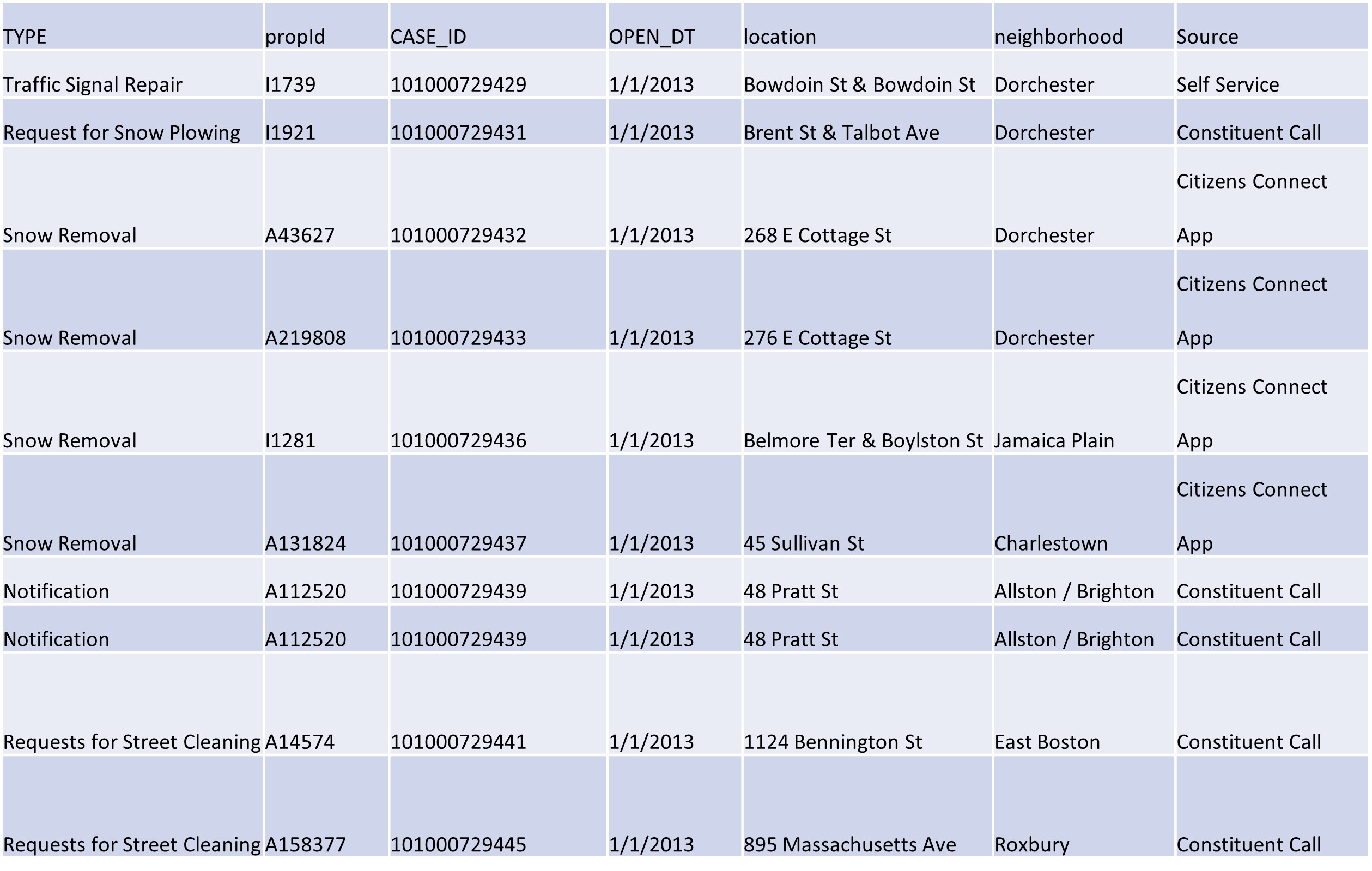
CRM[ncol(CRM),nrow(CRM)/2]nrow(CRM[CRM$neighborhood == 'Dorchester’ & CRM$TYPE == ‘Snow Removal’,])nrow(CRM[CRM$neighborhood == 'Dorchester’ | CRM$TYPE == “Snow Removal”,])
- Translate each of the following commands into
tidyverse.CRM[ncol(CRM),nrow(CRM)/2]nrow(CRM[CRM$neighborhood == 'Dorchester’ & CRM$TYPE == ‘Snow Removal’,])nrow(CRM[CRM$neighborhood == 'Dorchester’ | CRM$TYPE == “Snow Removal”,])CRM[order(CRM$neighborhood, CRM$TYPE),]
3.8.2 Exploratory Data Assignment
Import a data set of your choice into R. This is the first exploratory data assignment in this book that works with a full data set drawn from an outside source. It is suggested that to get the most from these assignments you use the same data set in all of them, though that is not required. Once you have imported the data set, complete the following:
- Briefly describe the structure of your whole data set or of some meaningful subset based one or more criteria (number of rows, columns, names of relevant variables).
- Describe at least three observations (rows) from this set/subset using the information contained in the variables you see as relevant.
- What have you learned from these observations individually, and from the differences between them?
- How do they illustrate what we can learn from these data more generally?
- Can you infer things about the observations that are not explicitly in the data?