5 Uncovering Information: Making and Creating Variables
“Life and health can never be exchanged for other benefits within the society.” So reads the mission statement for Vision Zero, a philosophy that treats pedestrian and cyclist deaths from automobile collisions not as inevitable events that should be reduced, but as tragedies that could be entirely eliminated by better design and management of roads. The idea was first introduced in Sweden in 1997, where traffic fatalities have since plummeted by over two-thirds. As of 2021, dozens of countries in Europe and cities in the United States and Canada have also adopted Vision Zero as a guiding principle in their transportation policy.
Vision Zero and the expanded use of data in public policy and practice—including in transportation—have evolved in tandem over the last two decades. But they have merged in the use of indicators for tracking a city’s success in eliminating traffic fatalities. San Francisco, for example, has a Transportation Safety Scorecard that includes traffic citations for the five violations responsible for the most collisions, including speeding, running stop signs, and disregarding the pedestrian right of way (e.g., ignoring a crosswalk; see top of Figure 5.1). New York City has a similar collection of metrics, also including their successes in revamping infrastructure, such as building new bike lanes, and outreach they have done around safety at schools and senior centers. Through these sorts of measures, cities can assess their progress, identify weak spots, and create awareness in the broader public.
Indicators have become a popular tool in urban informatics and are certainly not confined to questions of transportation. Indicators are central to performance management efforts that evaluate the effectiveness of operations across departments. These are often the basis of “dashboards” that can be part of a city’s open data portal or an internal interface for managers—or even the mayor—to quickly take stock of current conditions. There are also efforts to use indicators to guide social service provision, as embodied in the National Neighborhood Indicators Partnership , a learning network coordinated by the Urban Institute on the use of data to advance equity and well-being across neighborhoods (see bottom of Figure 5.1).
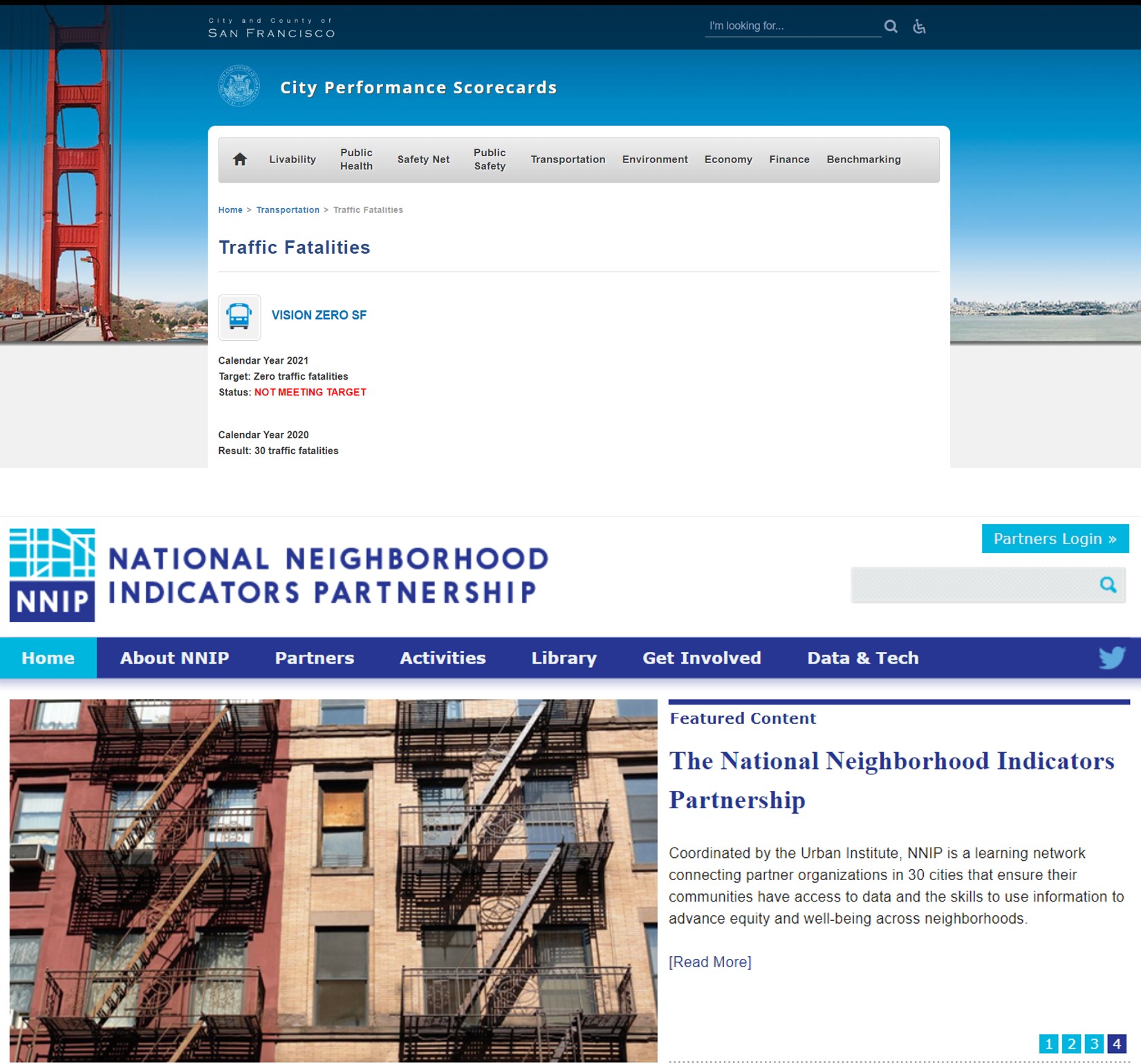
Figure 5.1: The City of San Francisco maintains a Transportation Safety Dashboard that tracks numerous metrics, including its goal of achieving zero traffic fatalities (i.e., Vision Zero; top). Meanwhile, National Neighborhood Indicators Partnership is an effort of the Urban Institute to coordinate partners in 30 cities all dedicated to the use of metrics to inform social service design and provision (bottom). (Credit: City of San Francisco, National Neighborhood Indicators Partnership)
The creation of indicators itself is a skill. An analyst—often in conversation with colleagues and community members—has to first determine, “What specifically do we want to know? What information needs to be tracked?” The answers to these questions are often lurking in the available data, but they need to be uncovered. This calls for numerous types of data manipulation: maybe tabulating relevant cases through the creation of categories, such as running stop signs; calculating one or more new variables or combining them, as in the case of an “opportunity index” that quantifies assets and deficits across communities; or even extracting content from lengthy descriptions of events through text analysis. Each of these processes (and others) help us to coax the desired information out of the data set. These are the skills we will learn in this chapter.
5.1 Worked Example and Learning Objectives
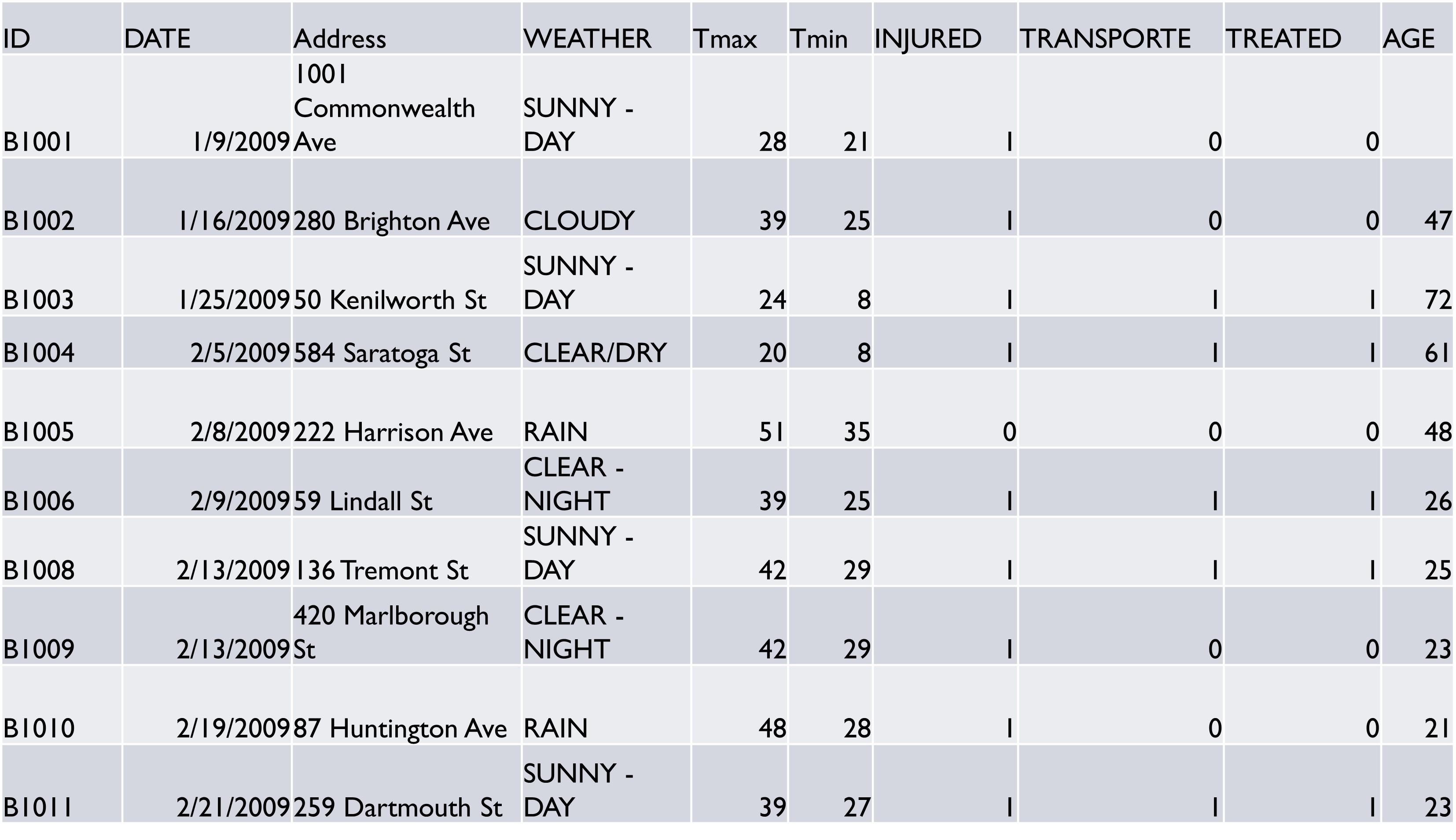
In this chapter, we will work with a database of bicycle collisions occurring in Boston from 2009 to 2012. The data were developed by Dahianna Lopez, who was a graduate student at the Harvard T.S. Chan School of Public Health at the time, through a series of internships with the Boston Police Department. She worked with raw police transcripts to extract numerous pieces of information about each collision, resulting in a detailed report on bicycle safety from the mayor’s office in 2014. The data were then published by the Boston Area Research Initiative .
These data give us an opportunity to observe the types of details that might be included in a data set to enable crucial indicators, like whether collisions resulted in medical treatment or transportation to a hospital. They also present the opportunity to manipulate data to create new variables (or simply edit old ones), thereby learning and practicing the following skills:
- Calculate numeric variables;
- Manipulate strings (often using the package
stringr); - Create categories based on criteria;
- Summarize and visualize the content of lengthy blocks of text;
- Work with date and time variables (using the package
lubridate); - Extend the ability to customize graphs in
ggplot2.
Link: https://dataverse.harvard.edu/dataset.xhtml?persistentId=doi:10.7910/DVN/24713. You may also want to familiarize yourself with the data documentation posted there.
Data frame name: bikes
bikes<-read.csv("Unit 1 - Information/Chapter 5 - Revealing Information/Example/Final Bike Collision Database.csv")
5.2 Editing and Creating Variables: How and Why?
There are three reasons why we might want to edit and create variables. Two speak to the tasks we can accomplish when working with variables. The third is the inspiration behind why we would want to manipulate variables in the first place.
- Adjusting issues that make analysis difficult. This could include errors in data entry that need to be fixed before we proceed. We saw in the previous chapter that some Craigslist postings have inexplicably low prices. We excluded them there by subsetting, but what if we want to replace them with NA’s instead? There might also be outliers that interfere with broader interpretations and we need to establish some “ceiling” or “floor” to the distribution of a variable. For instance, in some cases analysts will set incomes over some threshold to a single highest value (e.g., all incomes >$500,000 would be set to $500,000).
- Making certain information more accessible for analysis. This could entail reorganizing the content in a single variable—maybe recoding it to be more interpretable or translating a numerical variable into a series of categories. It might also entail combining information contained in multiple variables. Many indexes, in fact, involve summing or averaging a collection of sub-indicators. In such a situation, you might need to calculate the sub-indicators first and then combine them.
- Exposing the information you actually want. Analyses are driven by the decisions of the analyst. As such, you want to enter every analysis asking the question, “What do I want to know?” The answer to that question will determine what variables you will create, analyze, and visualize.
5.3 Variables in the Bike Collisions Dataset
Before we get going, let’s take a quick look at the data set so that we can decide what direction our analysis will take.
names(bikes)## [1] "ID" "YEAR" "DATE" "DAY_WEEK"
## [5] "TIME" "TYPE" "SOURCE" "XFINAL"
## [9] "Xkm" "YFINAL" "Ykm" "Address"
## [13] "Main" "RoadType" "ISINTERSEC" "TRACT"
## [17] "CouncilDIS" "Councillor" "PlanningDi" "OIF1"
## [21] "OIF2" "OIF3" "OIF4" "BLFinal"
## [25] "CS" "LIGHTING" "Indoor" "Light"
## [29] "LightEng" "WEATHER" "PrecipCond" "AtmosCondi"
## [33] "DayNight" "Tmax" "Tmin" "Tavg"
## [37] "Temprange" "SunriseTim" "SunsetTime" "SnowFall"
## [41] "PrecipTota" "Fault" "Doored" "HelmetDocu"
## [45] "TaxiFinal" "hitrunfina" "AlcoholFin" "INJURED"
## [49] "TRANSPORTE" "TREATED" "GENDER" "ETHNICITY"
## [53] "AGE" "Narrative"A quick glance at variable names (which could be confirmed by reading the data documentation published alongside the data) reveals that there are a lot of variables describing the weather, including temperature (Tmax, Tmin, Tavg, Temprange) and precipitation (PrecipCond, SnowFall, PrecipTota), and the circumstances surrounding the collision (Doored, TaxiFinal, hitrunfina), its outcomes (INJURED, TRANSPORTE, TREATED), and the characteristics of the biker (GENDER, ETHNICITY, AGE). There is also an extended police Narrative that we might want to leverage. As we move forward, we will look for ways to better specify the way the weather might have shaped the event and also to capitalize on the rich content of the police narrative.
5.4 Calculating (and Recalculating) Numeric Variables
We will start with functions that calculate numerical variables. Notably, any tool we learn here or throughout the chapter can create a “new” variable or recreate an old one by writing over it. The only distinction is the variable name that we indicate on the left side of the arrow. Overwriting can be risky, though. If we make a mistake, it can be difficult to recover the original content.
5.4.1 One Variable, One Equation
The simplest way to calculate a new variable in base R is by storing or assigning an equation to a new variable, using our friends <- and $. For instance, let’s say we want to know the average temperature in Celsius rather than Fahrenheit.
bikes$Cels_Tavg<-(bikes$Tavg-32)*5/9Note that this does not generate any output, but that the number of variables in bikes just increased from 54 to 55 in the Environment.
The new variable is Cels_Tavg (use names() if you would like to check). Let’s take a quick look at the variable using summary().
summary(bikes$Cels_Tavg)## Min. 1st Qu. Median Mean 3rd Qu. Max.
## -10.00 11.67 17.78 16.42 22.78 33.33Those values would seem to check out as plausible in a city like Boston. Now, if you were dedicated to analyzing the data in Celsius only and overwriting the existing Tavg variable, you could have done that by (note that I am not actually executing this command, just showing it):
bikes$Tavg<-(bikes$Tavg-32)*5/9These commands will store the output of any equation on the right side in the variable named on the left side. If that variable already exists, it will be overwritten.
5.4.2 Multiple Variables, One Equation
Tavg is not our only temperature variable. We also have a minimum and maximum. What if we want to convert them all to Celsius at once? First, let’s dispose of our newly created variable so that we can recalculate it as part of this new process:
bikes<-bikes[-55] #(i.e., remove column 55)Now we are ready to do this:
bikes[55:57]<-(bikes[c(34:36)]-32)*5/9Why does this work? Let’s unpack it, starting with the equation. We have subset bikes to columns 34-36. If you check with names(), these are the original temperature variables. We have then calculated the Fahrenheit-to-Celsius conversion on each of them and then stored them in three new columns, 55-57.
This type of calculation can be efficient from a coding perspective but is error prone. For instance, you will want to be confident you know the number of columns in your data frame (use ncol()). It also makes for code that can be difficult to replicate if there are slight differences between versions of data that change the order of variables. Nonetheless, it is important to know this is possible.
5.4.2.1 Renaming Variables
Take a look at names(). The last three variables are a little odd looking (e.g., Tmax.1, Tmin.1). We need to rename them if they are going to be meaningful. But how do we do that? It turns out that the names of a data frame are an editable object as well! Thus, names() not only tells us what the variable names are but also allows us to change them.
names(bikes)[55:57]<-c('Cels_Tmax','Cels_Tmin','Cels_Tavg')Thus, we have given each of these columns a name matching the original variable but with ‘Cels_’ in front of it.
5.4.3 Multiple Variables, Different Equations
What if we want to calculate multiple variables but each one requires its own equation? The transform() function is built for this very purpose. We still need to recreate our range variable in Celsius. But, for the sake of illustration, maybe we want to check that the average was calculated correctly while we are at it.
bikes<-transform(bikes,Cels_Temprange=Cels_Tmax-Cels_Tmin,
                 Cels_Avg=(Cels_Tmin+Cels_Tmax)/2)
transform() requires two arguments: the name of the data frame of interest and one or more variables to be calculated. Here we have calculated the range (max-min) and the average ((min+max)/2). Note that I have given the average variable a distinct name so that we do not overwrite the existing one. Also, though the output is the entire bikes data frame, transform() keeps all existing variables and adds only the new ones.
You can take a look at the range variable using summary(). And if you use View() you can see that our two average variables are identical (minus some occasional rounding). You can remove the new version if you like with the following code.
bikes<-bikes[-59]5.4.4 Calculating Variables in tidyverse
Next we want to learn how to do the same tasks in tidyverse (remember to require(tidyverse) for this segment). The single variable-single equation calculations do not require tidyverse, but the multiple calculations might benefit from it. It turns out that the mutate() command in tidyverse is almost identical to the transform() command.
bikes<-mutate(bikes,Cels_Temprange=Cels_Tmax-Cels_Tmin,
              Cels_Avg=(Cels_Tmin+Cels_Tmax)/2)
Because the first argument in the mutate() function is the name of the data frame of interest, it can be incorporated into piping, as in this trivial example:
bikes<-bikes %>%
  mutate(Cels_Temprange=Cels_Tmax-Cels_Tmin,
      Cels_Avg=(Cels_Tmin+Cels_Tmax)/2)
Note that, as we have seen in previous chapters, the argument bikes is not included in the mutate() command in the second line of the pipe because it is being drawn from the previous line. Also, note that we are replacing the bikes data frame with a new version that has all previous variables plus the new ones.
The one difference between transform() and mutate() is the ability of the latter to reference variables within it that do not yet exist. For example, we could rewrite the previous command:
bikes<-mutate(bikes,Cels_Temprange=Cels_Tmax-Cels_Tmin,
              Cels_Avg=Cels_Tmin+Cels_Temprange/2)
That is, the average is equal to the minimum plus half of the range. This might not be the most intuitive way to write this equation, but it illustrates an important capability of mutate() that can come in handy: one variable in the command can be calculated using another variable calculated in the same command. transform() would generate an error in this case because Cels_Temprange does not already exist in the bikes data frame.
5.5 Manipulating Character Variables: stringr
The most powerful tool for working with character variables, including factors, is the stringr package (Wickham 2019) . You likely will not need to install and require() it at this time because it is included as part of tidyverse.
stringr comprises a plethora of functions, including for mutating character values, also known as “strings” of text (i.e., systematically changing their values), joining and splitting strings, detecting matches, isolating and altering subsets of strings, and others. We will work through examples of the first three of these, but I also recommend you spend some time with the stringr cheat sheet that the folks at tidyverse have been kind enough to provide (https://github.com/rstudio/cheatsheets/blob/master/strings.pdf).
You will also want to familiarize yourself with “regular expressions,” also known as regex. These are on pg. 2 of the stringr cheat sheet. Regular expressions allow you to specify more general patterns, like something being at the beginning or end of a word, whether it is alphanumeric or only contains numbers, and others. We will avoid these in our examples here, but they can all be expanded with regular expressions.
5.5.1 Mutating Strings
Sometimes strings are messy. The simplest issue can be R’s sensitivity to capitalization. It is good practice to make your character variables all uppercase or lowercase before moving forward using the str_to_lower() or str_to_upper() functions.
bikes$WEATHER<-str_to_lower(bikes$WEATHER)
bikes$WEATHER<-str_to_upper(bikes$WEATHER)
Use the table() function after each command to see how the values have been mutated. We have overwritten the WEATHER variable with these lines of code, but we could also create two new variables using mutate().
bikes<-mutate(bikes,
          WEATHER_lower=str_to_lower(bikes$WEATHER),
          WEATHER_upper=str_to_upper(bikes$WEATHER))
5.5.2 Joining Strings
The str_c() is useful when we want to combine sets of strings. Importantly, it will align the strings of two vectors (i.e., lists of strings) of the same length, creating a vector of the same length as the first two.
For instance, we earlier created four new variables for temperature in Celsius. We named these variables according to a convention with ‘Cels_’ as a prefix to the previous variable name. str_c() can make this simpler by:
names(bikes)[55:58]<-str_c('Cels',names(bikes)[c(34:37)],sep='_')Let’s unpack this. The first argument was ‘Cels’. Because it is a single value, rather than a vector, it becomes a prefix for all values in the second argument, which is the names of variables 34-37 in bikes. Last, the sep= argument allows us to put a consistent separator between our arguments. The results are exactly what we would expect (you can check with names()) : Cels_Tmax, Cels_Tmin, Cels_Tavg, and Cels_Temprange.
str_c() will also work if the first argument were itself a vector, say, if we wanted a variable that combined the minimum and the maximum in one place
bikes$Cels_MinMax<-str_c(bikes$Cels_Tmin,bikes$Cels_Tmax,sep='-')Use summary() to see the results.
5.6 Creating Categories
Creating new categorical variables can be an effective way to simplify data and make it more immediately accessible to analysis. Here we will walk through three examples: categorizing by textual content, categorizing more general by any combination of criteria, and categorizing numerical variables by their levels.
5.6.1 Categorizing by Content: str_detect()
Let’s return to our WEATHER variable, which we will work with as being all uppercase. Take a look at the different values therein:
table(bikes$WEATHER)##
## CLEAR CLEAR-COLD
## 156 11 1
## CLEAR-DAY CLEAR-DAYLIGHT CLEAR-DRY-DAY
## 12 1 1
## CLEAR-MORNING CLEAR - CLEAR - DAY
## 1 2 7
## CLEAR - NIGHT CLEAR / DUSK CLEAR AFTERNOON
## 344 1 1
## CLEAR COOL CLEAR DAY CLEAR EVENING
## 1 7 1
## CLEAR NIGHT CLEAR SUNNY WARM CLEAR SUNNY WARM DAY
## 6 1 1
## CLEAR/DAY CLEAR/DRY CLOUDY
## 1 1 191
## CLOUDY/WET COOL AND CLEAR DARK
## 1 1 1
## DAY DAY - CLOUDY DAY/SUNNY
## 4 1 1
## DRIZZLE DRIZZLING DUSK
## 1 3 1
## FOG HEAVY RAIN HEAVY SNOW
## 1 2 1
## LIGHT RAIN N/A OTHER
## 1 4 8
## OVERCAST PARTLY CLOUDY RAIN
## 1 2 104
## RAIN - NIGHT RAINING RAINY, WINDY
## 1 1 1
## SLEET SNOW SNOW/SLEET/RAIN
## 2 10 1
## SPRINKLNG SUNN SUNNY
## 1 1 2
## SUNNY - DAY SUNNY - WARM SUNNY 75 DEGREES
## 689 1 1
## SUNNY DAY TORNADO UNKNOWN
## 3 1 4
## WARM WARM AND CLEAR WET
## 1 1 1There are a lot of different values. It might help us to simplify this list. For instance, there are numerous different versions of “CLEAR.” The str_detect() function can be useful here.
bikes$Clear<-as.numeric(str_detect(bikes$WEATHER, "CLEAR"))What did we do? str_detect has two arguments: the variable (or list of text) within which we are looking for text, and the text (or pattern) we are looking for. We have sought to find every value in bikes$WEATHER with “CLEAR” in it. str_detect() generates a logical (TRUE/FALSE) variable, so we convert it to a dichotomous numeric (0/1) variable.
table(bikes$Clear)##
## 0 1
## 1205 403There are 403 cases for which the description of the weather included the word “clear.” We could do the same for “rain,” which appears in a number of the descriptions.
bikes$Rain<-as.numeric(str_detect(bikes$WEATHER, "RAIN"))
table(bikes$Rain)
##
## 0 1
## 1497 111There are 111 cases for which the description of the weather included the word “rain.”
5.6.2 Categorizing by Criteria: ifelse()
Categorizing by content is one specific case of the broader ability of R to create categories based on specific criteria. This is crucial when creating custom variables and indicators as the analyst must decide what the criteria are that define the desired information.
The ifelse() function is able to translate criteria into new variables. It has three arguments: (1) the criterion or criteria of interest; (2) the result you want if the criteria are TRUE; (3) the result you want if the criteria are FALSE.
First, let us replicate our str_detect() command for bikes$Clear from above with ifelse().
bikes$Clear<-ifelse(str_detect(bikes$WEATHER, "CLEAR"),1,0)Instead of converting the result of str_detect() with as.numeric(), we stated that TRUE should be coded as 1 and FALSE as 0. This is a trivial example, but illustrates how ifelse() works.
We might expand our criteria. We know that the weather was described as clear, but does that guarantee that there was no recent precipitation and the street was dry? We might instead want the following
bikes$ClearNoPrecip<-ifelse(str_detect(bikes$WEATHER, "CLEAR")
                        & bikes$PrecipTota == 0, 1, 0)
table(bikes$ClearNoPrecip)
##
## 0 1
## 1322 286We now have only 286 cases for which this was true, down from 403.
We might go further, though, by nesting ifelse() commands to create a more nuanced but simplified weather variable.
bikes$WeatherCateg<-ifelse(str_detect(bikes$WEATHER, "CLEAR") &
                             bikes$PrecipTota == 0, "CLEAR",
                           ifelse(bikes$PrecipTota>0,
                                  "PRECIPITATION","CLOUDY"))
What did we do? The first ifelse() command includes our previous criteria, but the new value for TRUE is “CLEAR”. Then, instead of assigning a value to FALSE, we conduct another ifelse() on those remaining cases. If they have any precipitation, then the value is "PRECIPITATION". If not, the final value is “CLOUDY”. We have now created a three-category variable:
table(bikes$WeatherCateg)##
## CLEAR CLOUDY PRECIPITATION
## 286 714 6085.6.3 Categorizing by Levels
We can create categories by levels of numerical variable using ifelse() as we saw in the examples using bikes$PrecipTota. We might want to create more categories based on systematic splits in the data. A classic example of this is splitting a data set into its quartiles—that is, evenly splitting the data into four groups from highest to lowest. This is done with the ntile() function (which is from the dplyr package in tidyverse).
bikes$Tavg_quant<-ntile(bikes$Tavg,n=4)This divides the average temperature variable into four evenly sized groups by their order.
table(bikes$Tavg_quant)##
## 1 2 3 4
## 402 402 402 402You could do the same thing with any other n—if you want 5, 10, 100 groups, you simply need to alter the n= argument.
5.7 Text Analysis
If we want to take our efforts on categorizing data to the next level, we might pursue text analysis, also known as text mining. This is when an analyst explores a large corpus of text for patterns, especially quantifying which words and combinations of words are the most common. This is a bit more advanced of a topic than most of the other content in this chapter, but for those who are interested you should be perfectly capable of following along and replicating this example based on what you have learned so far.
This section will use the tm (Feinerer and Hornik 2020) package, which was designed for text mining, to work through five steps:
- Preparing the data
- Creating a corpus, or analyzable body of text
- Cleaning the text
- Creating a document term matrix, or the frequency of each word in each record in the corpus
- Tabulating word frequencies
We will use the products of Step 5 to then inform new categorical variables that might otherwise have been just guessing at.
require(tm)5.7.1 Step 1: Preparing the Data
The first step is to make sure that your data is ready to be analyzed. We want to analyze the variable Narrative as it has such rich content. It is a character variable (check using class()), which is what we need. If you take a quick look at the content, though (using head() or View()) you will notice a lot of strings of x’s. This is because the data were redacted to remove any potentially identifiable information about the individuals in the collision. We want to eliminate all of these using str_replace_all(), which searches a particular set of text for a certain pattern of text and then replaces it with another pattern of text.
bikes$Narrative <- str_replace_all(bikes$Narrative, "xx", "")
bikes$Narrative <- str_replace_all(bikes$Narrative, "xxx", "")
bikes$Narrative <- str_replace_all(bikes$Narrative, "xxxx", "")
bikes$Narrative <- str_replace_all(bikes$Narrative, "xxxxx", "")
bikes$Narrative <- str_replace_all(bikes$Narrative, "xxxxxx", "")
bikes$Narrative <- str_replace_all(bikes$Narrative, "xxxxxxx",
                                   "")
bikes$Narrative <- str_replace_all(bikes$Narrative, "xxxxxxxx",
                                   "")
bikes$Narrative <- str_replace_all(bikes$Narrative, "x ", "")
bikes$Narrative <- str_replace_all(bikes$Narrative, "the", "")
bikes$Narrative <- str_replace_all(bikes$Narrative, "THE", "")
To illustrate, the first line searched bikes$Narrative for every instance of “xx” and replaced it with “”, meaning a blank space. We also want to remove the word “the.” While this might not be what we want if we were going to read something, it is okay here because we simply want R to be able to see all of the words.
5.7.2 Step 2: Creating a Corpus
Next, we need to create a corpus. What is a corpus? It is a collection of individual pieces of text in a workable format. These pieces of text are more or less organized as the elements of a vector, but in a unique structure that enables the commands of the tm package to be most efficient. Creating the corpus is where we will first use the functionality of tm with the VectorSource and VCorpus functions.
my_corpus <- VCorpus(VectorSource(bikes$Narrative))Note that the class of my_corpus is indeed specific to tm:
class(my_corpus)## [1] "VCorpus" "Corpus"If you try to print my_corpus, you will not get very much information back. But you can look at individual cases with writeLines.
writeLines(as.character(my_corpus[[100]]))On at app Officer , x, responded to a r/c for a pedestrian struck by a m/v at Rd and Dudley St. Dispatch states that x, x, and are already on scene.
Upon arrival Officer spoke to Officer , x, who states that victim was riding his bike down St and entered intersection of Rd and St and was struck by Mass reg . Officer furr states that victim had a strong odor of alcohol coming from his breath. Officer states that victim suffered an injured left leg and was transported by H+H Amb to BMC. Officer states that victim told her that he had green light on St and as he entered intersection, car came down Rd and hit him.
Officer spoke to operator of Mass reg , Butler, who stated he was driving down Rd, he had green traffic light at St, he entered intersection of Rd and St and he was almost through intersection when a man on a bicycle came out of St, and drove right in front of his m/v and that he struck man on bike. Officer observed passenger side of windshield smashed.
The text here is that of the narrative from the 100th row.
5.7.3 Step 3: Cleaning the Text
Now that we have a corpus, we can start to work with it. Our next step will be to clean the text. You may be thinking, “Didn’t we already get rid of all of the redacted text?” Yes, but there’s a lot more to do to make the corpus intelligible for analysis. This will all be done with the tm_map() function, which takes the corpus in question and applies one of a variety of transformations to it.
We need to:
- Remove punctuation:
my_corpus <- tm_map(my_corpus, (removePunctuation)) - Remove numbers:
my_corpus <- tm_map(my_corpus, (removeNumbers)) - Remove stop words, like “a”, “the”, “is”, and “are”, which are very common but contain little information:
my_corpus <- tm_map(my_corpus, content_transformer(removeWords), stopwords("english")) - Replace hyphens with spaces, so that the pieces of a hyphenated word can be observed separately:
my_corpus <- tm_map(my_corpus, content_transformer(str_replace_all), "-", "") - Transform to lower case for consistency:
my_corpus <- tm_map(my_corpus, content_transformer(tolower)) - And remove unnecessary spaces:
my_corpus <- tm_map(my_corpus, (stripWhitespace)).
my_corpus <- tm_map(my_corpus, (removePunctuation))
my_corpus <- tm_map(my_corpus, (removeNumbers))
my_corpus <- tm_map(my_corpus, content_transformer(removeWords),
                    stopwords("english"))
my_corpus <- tm_map(my_corpus,
                content_transformer(str_replace_all), "-", " ")
my_corpus <- tm_map(my_corpus, content_transformer(tolower))
my_corpus <- tm_map(my_corpus, (stripWhitespace))
Let’s see what row 100 reads like now.
writeLines(as.character(my_corpus[[100]]))on app officer x responded rc pedestrian struck mv rd dudley st dispatch states x x already scene upon arrival officer spoke officer x states victim riding bike st entered intersection rd st struck mass reg officer furr states victim strong odor alcohol coming breath officer states victim suffered injured left leg transported hh amb bmc officer states victim told green light st entered intersection car came rd hit officer spoke operator mass reg butler stated driving rd green traffic light st entered intersection rd st almost intersection man bicycle came st drove right front mv struck man bike officer observed passenger side windshield smashed
It is essentially a list of meaningful words without the intervening words and punctuation that make text readable, like punctuation, stop words, etc. But this is exactly what we want for text mining. These words are the basis for the analysis to follow.
5.7.4 Step 4: Creating a Document Term Matrix
We now need to create a new object called a document term matrix (of class DocumentTermMatrix). The document term matrix converts the corpus into a table that counts the incidences of each word in each item in the corpus. Let’s create one from our corpus and then use the inspect() command to see what this means in practice for five rows.
dtm_bike <- DocumentTermMatrix(my_corpus)
inspect(dtm_bike[1:5,])
## <<DocumentTermMatrix (documents: 5, terms: 3088)>>
## Non-/sparse entries: 366/15074
## Sparsity : 98%
## Maximal term length: 19
## Weighting : term frequency (tf)
## Sample :
## Terms
## Docs and bicycle front left motor observed officer officers
## 1 6 1 2 0 3 1 4 0
## 2 0 1 0 2 0 0 2 0
## 3 0 2 1 0 0 2 5 0
## 4 0 1 1 2 0 0 0 1
## 5 0 4 3 4 12 6 7 8
## Terms
## Docs stated vehicle
## 1 4 5
## 2 3 0
## 3 3 2
## 4 0 0
## 5 6 12Reading this table, we can see that the document we have been looking at, row 100, contains the word “officer” 8 times, as does row 103. The word also appears in all three other cases. One might infer that row 103 involved an illegal action as the word “suspect” occurs 10 times and “victim” occurs 9 times. Overall, this is a simple way to interact with the content of the corpus.
The top of the output can also be useful. We have limited to five documents here that across them have 3,088 different terms (or words). The sparsity analysis tells us how consistent these terms are across documents. Of the 15,440 possible document-term combinations (3,088*5), only 329 are true. This makes sense-—3,088 terms is a lot of terms, and only some of them will repeat often, and many will be specific to the given case. If, however, we had a corpus with fewer total terms that were expected to be consistent across documents, we would expect lower sparsity.
5.7.5 Step 5: Examining Word Frequency
Oddly, to really analyze our word frequencies, we are better off converting the document term matrix into a data frame, summing across all columns to calculate the frequency of every term present in the corpus.
words_frequency<-data.frame(colSums(as.matrix(dtm_bike)))This multi-function command does more or less what we want, but using the View() command, you might note that it is a little strange looking. There is no variable for the terms, but instead the terms are the names of the rows. The column has a funny name.
We want to pretty this up by:
- Creating a new variable for the term:
words_frequency$words <- row.names(words_frequency) - Renaming the frequency column:
names(words_frequency)[1] <- "frequency" - Renaming the rows as numbers, which is more common:
row.names(words_frequency) <- 1:nrow(words_frequency) - and flipping the order of out variables to the more customary setup of terms followed by frequencies:
words_frequency <- words_frequency[c(2,1)].
Now that we have this, we can look more closely at the frequency of certain words. Are words about weather common?
words_frequency$words<-row.names(words_frequency)
names(words_frequency)[1] <- "frequency"
row.names(words_frequency)<-1:nrow(words_frequency)
words_frequency<-words_frequency[c(2,1)]words_frequency[words_frequency$words == "rain",]## words frequency
## 2077 rain 9Only 9 cases of the word rain! What if we use str_detect() to look for any word containing the text “rain”, which could then include “rainy”, “rainstorm”, or otherwise.
words_frequency[str_detect(words_frequency$words, "rain"),]## words frequency
## 1647 moraine 6
## 2077 rain 9
## 2078 raining 3
## 2722 train 10Here we see the potential weakness of this approach without paying close attention—“moraine” (which is a street name) and “train” are included as well.
If we look at the word “clear” we get 14 instances, but that could also include statements like, “The road was clear.”
Meanwhile, the most frequent words appear to be more about the actors in the collision and its resolution.
head(arrange(words_frequency,-frequency), n=10)## words frequency
## 1 victim 5386
## 2 officer 4929
## 3 stated 4709
## 4 vehicle 3627
## 5 bicycle 2917
## 6 and 2752
## 7 was 2184
## 8 struck 2134
## 9 the 2093
## 10 street 1841We see here that some of the most common words are “victim” (5,386), “officer” (4,929), “vehicle” (3,627), and “bicycle” (2,918).
5.7.6 Summary and Usage
We have now tabulated the frequency of every word in the full corpus of police narratives on bicycle collisions in Boston for 2009-2012. This makes that information much more accessible, and anything we do with it better informed. We might use the list of frequent terms or a search for terms with similar content to create new, better-informed categorical variables. You are welcome to take a break from the book and go play with this now. We can also visualize these frequencies to better communicate them, which we will do in Section 5.9.3.
5.8 Dealing with Dates
Date and time variables come in many classes and can be quite tricky to work with. This is because of the many ways that one might organize this sort of information—date, date followed by time, time followed by date, month and year only, and time only are just a handful of examples. And then there are questions like whether the time has seconds or not, whether it includes time zone, whether the date is month-day-year or day-month-year, etc. Luckily, the package lubridate makes this much more straightforward (Spinu, Grolemund, and Wickham 2021). Here we will focus specifically on analyzing dates.
First, we need to convince R that we have date data. Currently, it thinks that the DATE variable is a character (check with class()). But if we print the content, it looks like a date of the form year-month-day. lubridate has a series of functions for converting characters that are intended to be dates to be recognizable in the appropriate format. Here we need ymd() for year-month-day.
require(lubridate)
ymd(bikes$DATE)[1]
## [1] "2009-01-25"We can then use a series of commands to extract the details of the date:
day(ymd(bikes$DATE))[1]## [1] 25month(ymd(bikes$DATE))[1]## [1] 1year(ymd(bikes$DATE))[1]## [1] 2009wday(ymd(bikes$DATE))[1]## [1] 1Most of these generate information we already knew from the date itself, but it isolates that information for further analysis. wday() does add something in that it identifies the day of the week, in this case it was a Sunday. We could also use this with ifelse() to create a new variable for collisions on weekends.
bikes$Weekend<-ifelse(wday(ymd(bikes$DATE))==1 |
                  wday(ymd(bikes$DATE))==7,
                  'Weekend', 'Weekday')
table(bikes$Weekend)
##
## Weekday Weekend
## 1262 346We can also calculate differences between dates. For example, if we want to determine the full range of the corpus, we might try the following
max(ymd(bikes$DATE))-min(ymd(bikes$DATE))## Time difference of 1427 daysThat is, we subtract the earliest date (the minimum) from the latest date (the maximum) and find that it is about 4 years long (which we knew based on the 2009-2012 time range).
It is also possible to calculate new date variables using lubridate with equations, though we have no immediate use for this here. A simple example could be adding three days onto any event.
head(ymd(bikes$DATE)+days(3))## [1] "2009-01-28" "2009-02-08" "2009-02-11" "2009-02-12"
## [5] "2009-02-16" "2009-02-16"5.9 Returning to ggplot2
The spirit of this chapter has been to manipulate variables to expose the precise information that we want to learn from. Apart from the text mining, we have not engaged with many new data structures. Thus, our learning of ggplot2 will move forward primarily to customize how we create our graphs as we get to know our content a bit better. The one exception to this will be in Section 5.9.3 when we learn how to visualize our text analysis in word clouds using the package wordcloud (Fellows 2018).
5.9.1 Visualizing Weather and Injuries – Customizing Graphs
The goal of Vision Zero is to eliminate serious injuries and fatalities from vehicle collisions. Let’s visually explore the relationship between injuries and the weather in this dataset. First, we have to set aside cases for which bikes$Injured == 99, which is often used in data to represent missingness.
base.no.na<-ggplot(bikes[bikes$INJURED!=99,], aes(x=Tavg))
Remember that the first step of working in ggplot2 is a command that establishes the basis for the graph but does not actually create the graph. We will now build upon base.no.na.
base.no.na+geom_histogram(aes(fill=as.factor(INJURED)))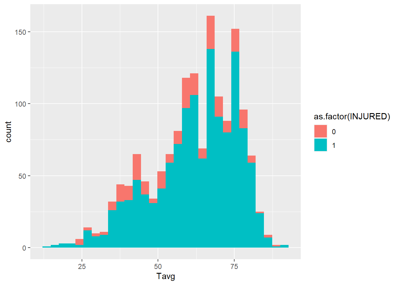 This is a nice graph, but it’s not perfect. We might improve it by adding a series of operations to our
 ggplot2 command:
- Make things a bit smoother with smaller bins of 5 degrees each with the
binwidth=argument:geom_histogram(aes(fill=as.factor(INJURED)), binwidth=5) - Rename the x-axis with
scale_x_continuous(), while also setting the range to 20⁰-90⁰ withlimits=, and making the labels every ten degrees with breaks= :+ scale_x_continuous("Average Temp.", limits = c(20,90), breaks = c(20,30,40,50,60,70,80,90)) - and rename the legend with
labs():+ labs(fill = "INJURED")
The whole thing looks like this:
base.no.na+
geom_histogram(aes(fill=as.factor(INJURED)), binwidth=5) +
scale_x_continuous("Average Temp.", limits = c(20,90),
               breaks = c(20,30,40,50,60,70,80,90)) +
  labs(fill = "INJURED")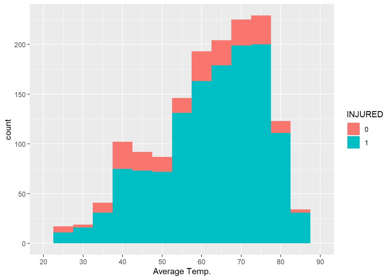
Now that we have the graph we want, we can take a closer look. In most cases there was an injury. It is not obvious, though, whether injuries were more common at some temperatures than others. It is possible that they were more common when it is very hot or very cold, but this graph does not definitively show that.
Before we move on, we are now going to save our current graph as a new object, full_graph.
full_graph<-base.no.na+
  geom_histogram(aes(fill=as.factor(INJURED)), binwidth=5) +
  scale_x_continuous("Average Temp.", limits = c(20,90),
                     breaks = c(20,30,40,50,60,70,80,90)) +
  labs(fill = "INJURED")
5.9.2 Visualizing a Third Variable: Facets
We have learned how to bring categorical variables in with the fill= argument. Another option is faceting, or creating the same graph repeatedly for all values of a categorical variable. Let’s suppose we want to split our temperature-injury analysis by precipitation conditions:
full_graph+facet_wrap(~WeatherCateg)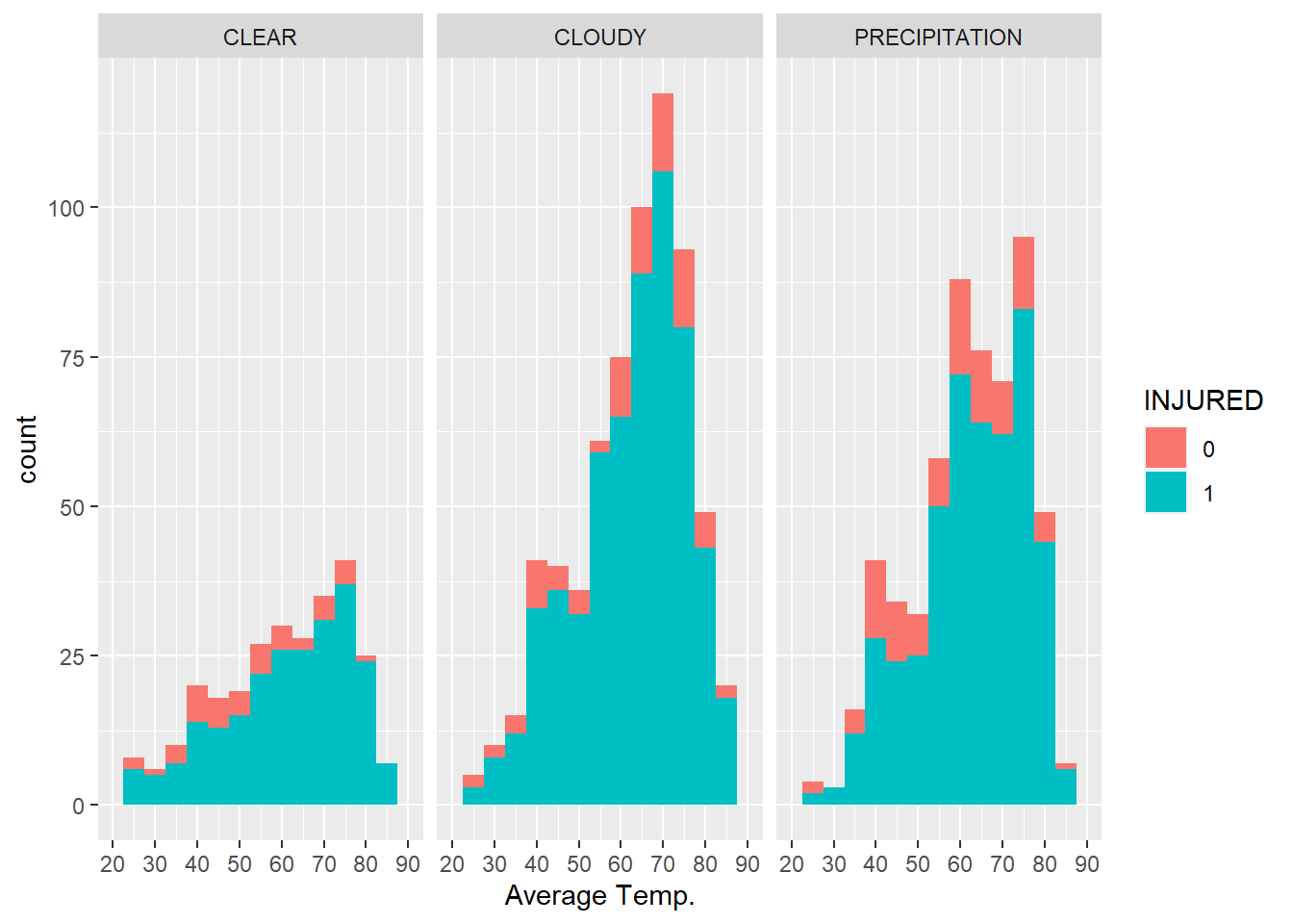
We could even go crazy and want to split by precipitation conditions and whether it was a weekend. This is possible with the facet_grid() command.
full_graph+facet_grid(WeatherCateg~Weekend)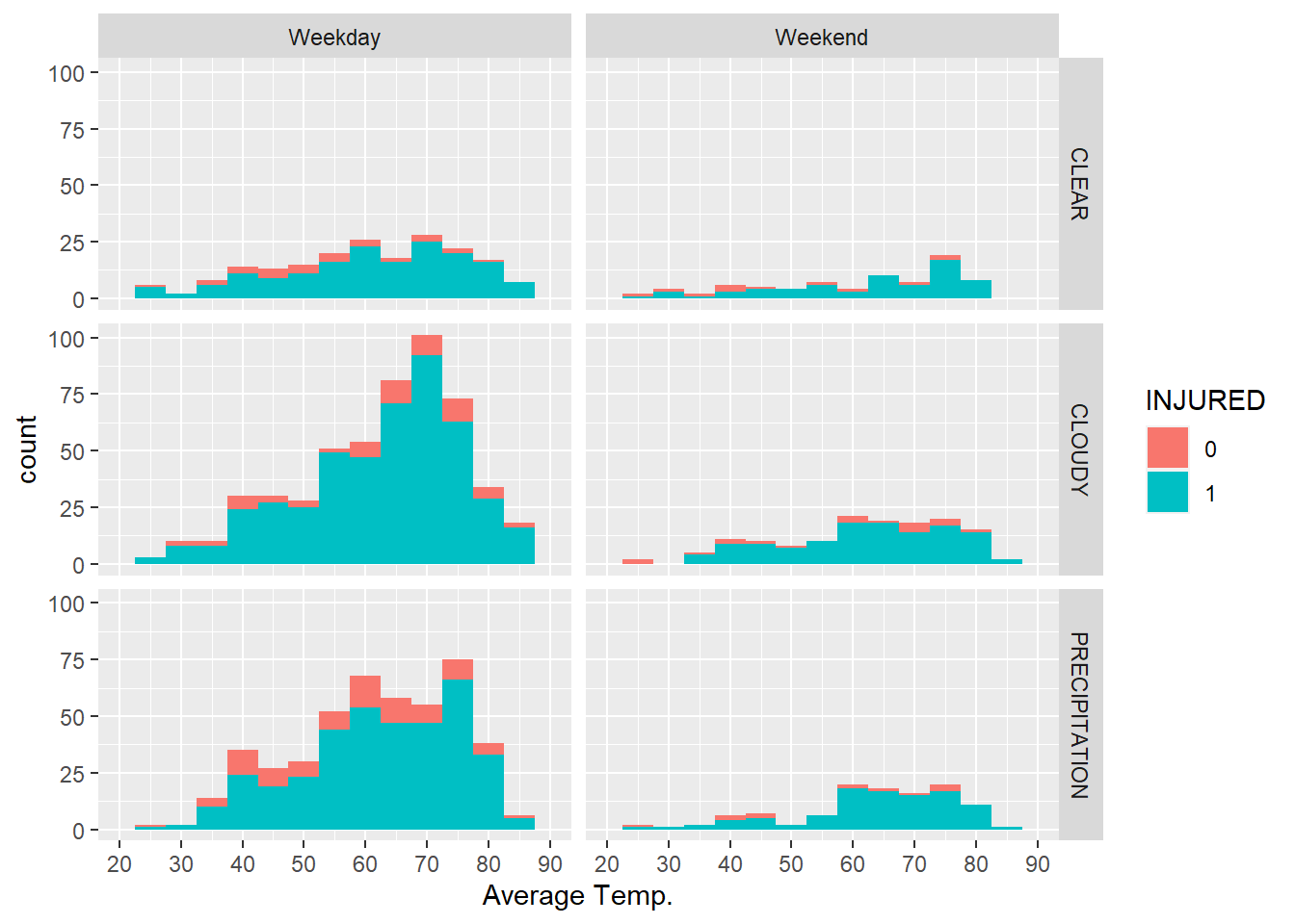
Interestingly, neither of these graphs communicates anything obvious about the relationship between injuries from collisions and weather. This reflects the concern that, regardless of the conditions, a collision between a car and a bicycle will almost always result in an injury for the bicyclist.
5.9.3 Visualizing Word Frequencies: Word Clouds
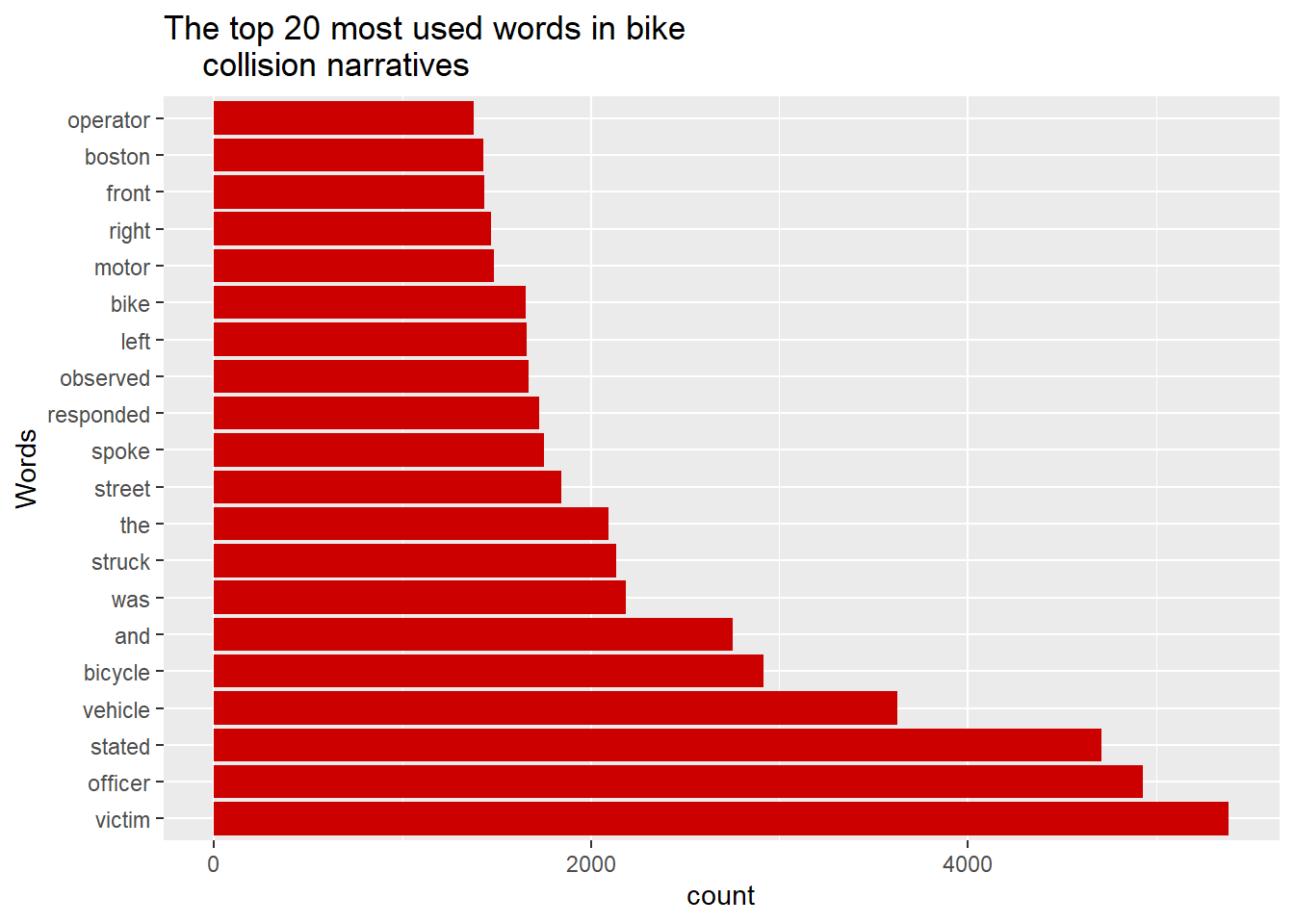
Remember the table of word frequencies we created from the police narratives? Provided you are in the same project, you should still have it in your Environment as words_frequency. We have all the tools we need to make a simple bar graph. Because we will want to limit the content—-2,971 words are way too many to visualize—we will use pipes.
pp <- words_frequency %>%
  arrange(desc(frequency)) %>%
  head(n=20) %>%
  ggplot(aes(x = reorder(words, -frequency), y= frequency)) +
  geom_bar(stat = "identity", fill = "red3") +
labs(title = "The top 20 most used words in bike
    collision narratives",
             x = "Words", y = "count") +
  coord_flip()
To explain what is happening here, the first three lines sort the data set by frequency with arrange() and then select the first 20 rows with head(), meaning the graph that follows will only visualize those 20 words. The ggplot() command then pre-orders our words by frequency, creates a bar graph (with stat=’identity’ instructing the graph to represent the y-value associated with each x and fill= setting a custom color), customizes the labels with labs(), and flips the coordinates to make the graph more readable with coord_flip(). The product is:
This is nice, but could we present the same information in a more engaging way? You may be familiar with word clouds, a graphic that represents the most common words in a corpus and sizes them proportional to their frequency. It is a fun and easily interpretable way of representing the prominent words in a corpus. This will require an additional package, wordcloud. You will need to install it.
require(wordcloud)
wordcloud(words = my_corpus, min.freq = 1, max.words=200,
      random.order=FALSE, rot.per=0.35,
      colors=brewer.pal(8, "Dark2"))
Unpacking this command, we have specified my_corpus as the source for words=; we have limited to words that appear at least once (min.freq) and to no more than the 200 most common words (max.words); we have turned off the random.order= option, which would grab words at random rather than by the order of their frequency; the rot.per= controls how many words are rotated to fit together; and the colors= command jazzed it up a bit (otherwise it would have been black and white). The product is:
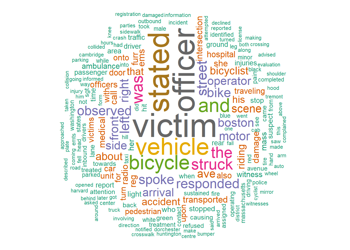
This image tells the story we largely already knew about the content of the corpus, but for someone who has not worked through it as thoroughly as we just did, it quickly highlights that the most common words center on the actors involved in the collision and its reporting—the victim, officer, vehicle, bicycle, and operator.
5.10 Summary
This chapter has worked through the creation of variables of various types using a database of bike collisions reported by the Boston Police Department from 2009 to 2012. We have focused on weather and, in the end, its relationship with injuries from collisions. In doing so, we have practiced the conceptual skill of thinking through the questions, “What do we want to know? How do we manipulate the data to expose that information?”
We practiced multiple technical skills for calculating variables, including:
- Calculated numerical variables in multiple ways:
- One variable, one equation with
<-and$notation, - Multiple variables, one equation with
[]notation, - Multiple variables, multiple equations with
transform()andmutate(), the latter being part of thetidyverse;
- One variable, one equation with
- Manipulated character variables with the package
stringr, including:- Mutating strings to be easier to analyze,
- Joining strings into a single varible;
- Created new categorical variables based on:
- Text elements with
str_detect(), - More general criteria with
ifelse(), - Quantiles of numerical variables with
ntiles();
- Text elements with
- Conducted text mining with the
tmpackage, - Dealt with dates with the
lubridatepackage, - Customized graphs in
ggplot2, including the incorporation of facets, - Created a wordcloud based on word frequencies using the
wordcloudpackage.
5.11 Exercises
5.11.1 Problem Set
- Assume that we are working with the following data frame titled
bikes. What would be generated for each of the following commands?
 a.
a. bikes$TRange<-bikes$Tmax-bikes$Tmin
bikes$TRange[6]
b. sum(str_detect(bikes$WEATHER,’SUNNY’))
c. bikes <-mutate(bikes,Tavg=(Tmax+Tmin)/2)
bikes$Tavg[3]
d. day(ymd(bikes$DATE))[1] + month(ymd(bikes$DATE))[2] + year(ymd(bikes$DATE))[3]
- Using the data frame
bikesfrom the worked example, write code to create each of the following categorizations. Check your work by executing the code and running tables on the resultant variables in R.- Average temperature was below freezing.
- Temperature was below freezing at any time.
- A categorical variable for no precipitation, rain, and snow.
- Whether the narrative referenced the driver as a “suspect.”
- Split precipitation by quartiles. Bonus: Do you think this is a useful variable? Why or why not? (Hint: Look at the values in each of the four quartiles.)
- Write code for creating each of the following variables. These are general and could be applied to any data frame. If it is easier, describe the steps that you would do in place of or alongside the code.
- You have a date variable. You want to create a variable for season.
- You have a ‘comments’ field. You want to flag for each case whether Boston is mentioned.
- You have a variable for day vs. night (0/1) and weekend vs. weekday (0/1). You want a single variable for weekend night.
- You want a text variable for all four categories—weekend day and night, weekday day and night.
- You have a date variable and want to isolate the year. i.The computer won’t recognize it as a date format.
5.11.2 Exploratory Data Assignment
Working with a data set of your choice:
- Create at least three new variables, each of which must either,
- Make some angle of your data’s content more interpretable, or
- Fix some issue in the data. Make sure to explain why these variables are useful.
- Describe the contents of these variables using analysis and visualization tools learned in this chapter and Chapter 4.